%load_ext notexbook
%texify -v
2.0.1).
Theme Settings:
- Notebook: Computer Modern font; 16px; Line spread 1.4.
- Code Editor:
Fira Codefont;14px; Material Theme. - Markdown Editor:
Hackfont;14px; Material Theme.
Solving Galactic Diffusion Equation using Crank Nicholson (W/O Ghost Zones)#
This notebook will illustrate the crank nicholson difference method solving Galactic Dynamo Diffusion Equation.
The implicit Crank-Nicolson difference equation of the Dynamo equation is derived by discretizing the following coupled equations
Where \(\eta_t\) is currently constant parameter called the magnetic diffusivity.
import numpy as np
import tabulate
from PIL import Image

import matplotlib.pyplot as plt
import scienceplots
plt.style.use(['science', 'notebook', 'grid'])
from matplotlib.animation import FuncAnimation
from IPython import display

from matplotlib import rcParams
rcParams['axes.grid'] = True
rcParams['grid.linestyle'] = '--'
rcParams['grid.alpha'] = 0.5
%matplotlib inline

import warnings
warnings.filterwarnings("ignore")
Discrete Grid#
Spatial Discretization:
We divide the spatial domain \(z\) into \(N\) grid points. Let \(h\) denote the spacing between consecutive grid points.
Time Discretization:
We discretize the time domain \(t\) into time steps of size \(k\).
The region \(\Omega\) is discretised into a uniform mesh \(\Omega_h\). In the space \(x\) direction into \(N\) steps giving a stepsize of
resulting in
and into \(N_t\) steps in the time \(t\) direction giving a stepsize of
resulting in
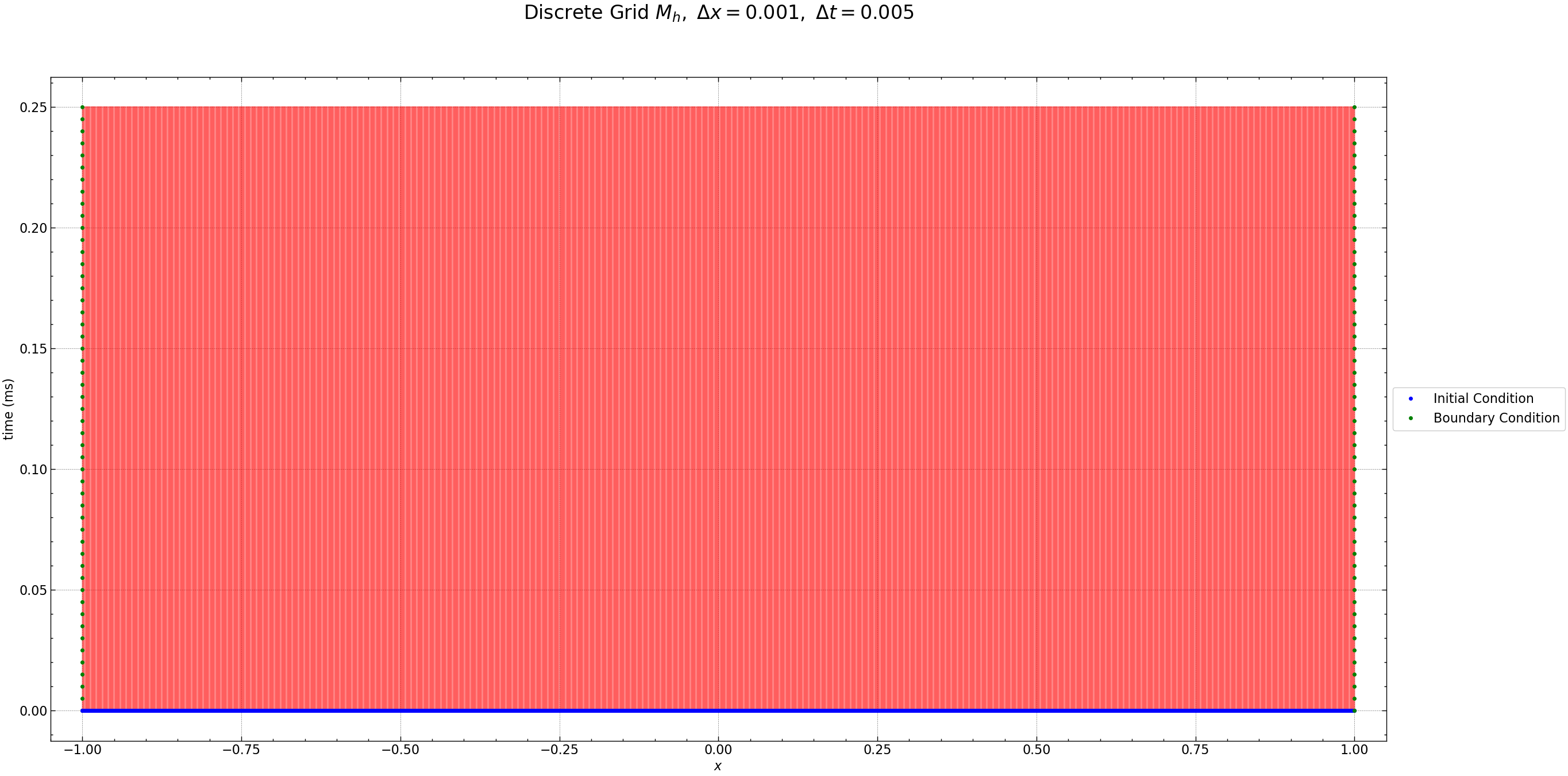
The Figure below shows the discrete grid points for \(N\) space points and \(N_t\) time points , the red dots are the unknown values, the green dots are the known boundary conditions and the blue dots are the known initial conditions of the diffusion Equation.
N = 2000
Nt = 400
h = 2 / N
k = 2 / Nt
r = k / (h * h)
eta_t = 1 # diffusion coefficient
time_steps = 50
time = np.arange(0, (time_steps + 0.5) * k, k)
z = np.arange(-1.00, 1.0001, h)
Z, Y = np.meshgrid(z, time)
fig = plt.figure(figsize=(30, 15))
plt.plot(Z, Y, 'r-', alpha=0.3)
plt.plot(z, 0 * z, 'bo', markersize=4, label='Initial Condition')
plt.plot(np.ones(time_steps + 1) * -1, time, 'go', markersize=4, label='Boundary Condition')
plt.plot(z, 0 * z, 'bo', markersize=4)
plt.plot(np.ones(time_steps + 1) * 1, time, 'go', markersize=4)
plt.xlim((-1.05, 1.05))
plt.xlabel(r'$x$')
plt.ylabel(r'time (ms)')
plt.legend(loc='center left', bbox_to_anchor=(1, 0.5))
plt.title(r'Discrete Grid $M_h,$ $\Delta x= %s,$ $\Delta t=%s$' % (h, k), fontsize=24, y=1.08)
plt.grid(True, linestyle='--', alpha=0.5)
plt.savefig("seed_1/grid.pdf")
plt.show()
Seed 1: Oscillatory Solution
Initial and Boundary Conditions#
Vacuum Boundary Conditions#
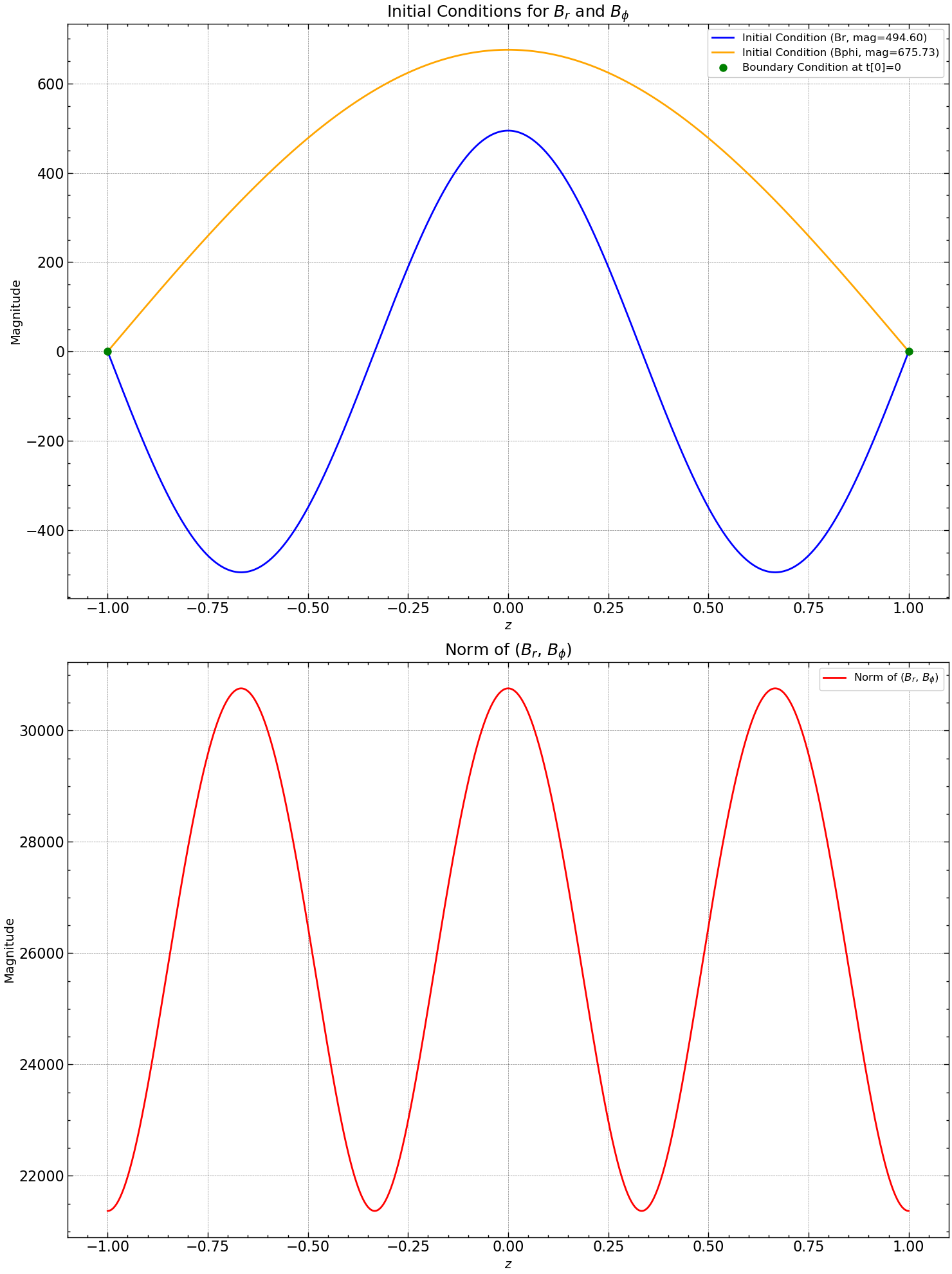
At \(|z| = h\) for a disc-shaped magnetized system, continuity of magnetic field components requires \(B_{\phi} = 0\) and \(B_r \approx 0\) at \(z = \pm h\). These exact conditions, known as vacuum boundary conditions, are due to axial symmetry and the outer magnetic field’s potential structure.
Discrete Initial and Boundary Conditions#
Discrete initial conditions:
Discrete boundary conditions:
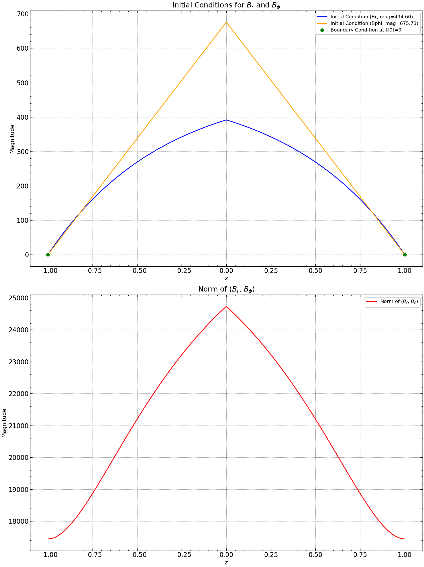
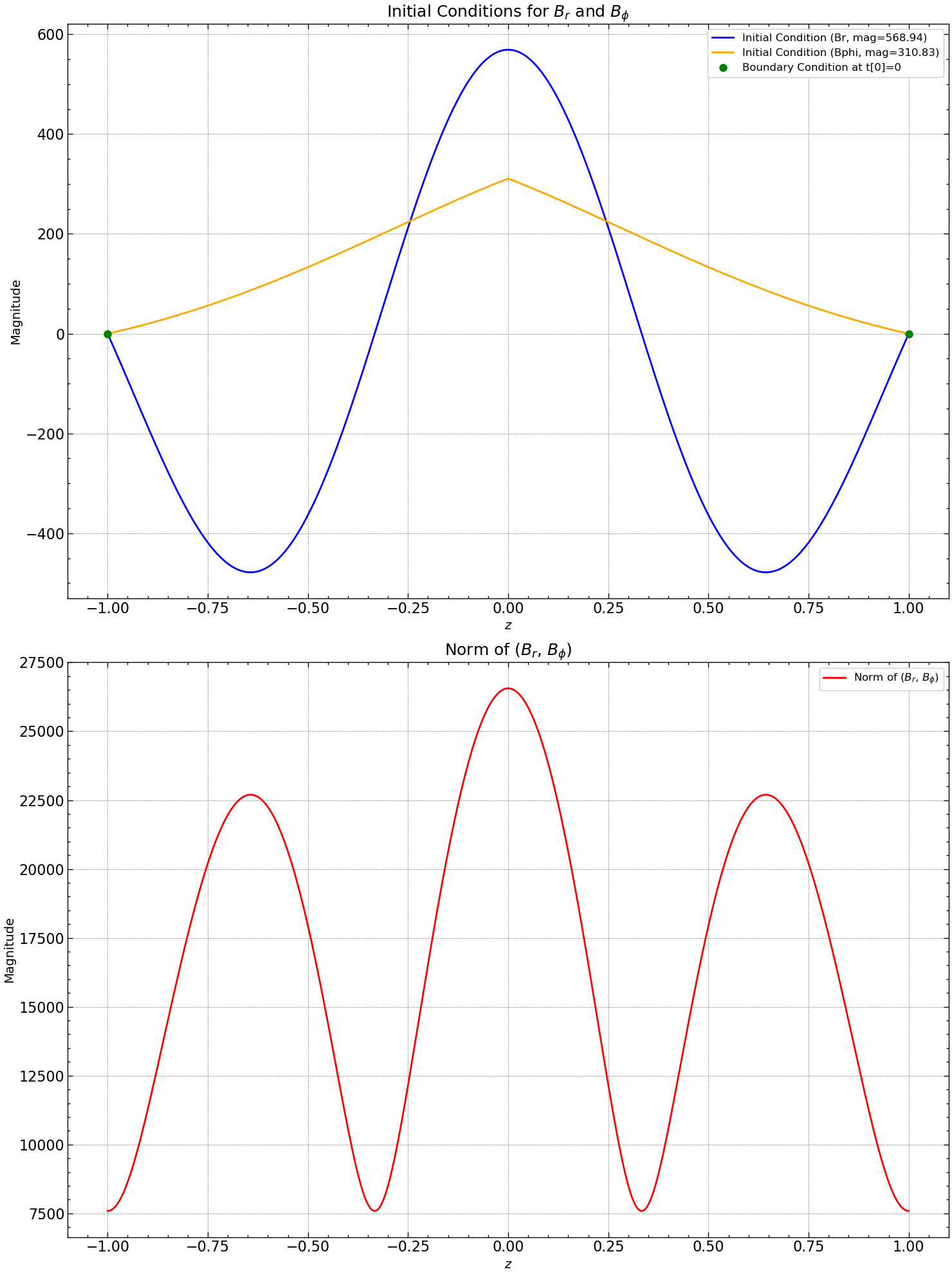
Here, \(B[i,j]\) represents the numerical approximation of \(B(x[i],t[j])\). For the case 1, we are looking at the exact eigensolution as seed field for \(B\) at \(t=0\), ensuring physical accuracy. The figure below displays \(B[i,0]\) for the initial (blue) and boundary (red) conditions at \(t[0]=0\).
def generate_random_Bo(seed_value):
    np.random.seed(seed_value)
    random_float = np.random.rand()
    return random_float

def initial_conditions(N, time_steps, seed_value, m, n, BCtype = "vacuum"):
    mag_br = 1000*generate_random_Bo(seed_value)
    mag_bphi = 1000*generate_random_Bo(seed_value + 1)

    z = np.linspace(-1, 1, N+1)
    Br = np.zeros((N+1, time_steps+1))
    Bphi = np.zeros((N+1, time_steps+1))
    b1 = np.zeros(N-1)
    b2 = np.zeros(N-1)

    # Initial Condition for Br and Bphi
    for i in range(1, N+1):
        Br[i, 0] = mag_br * np.cos((m + 1/2) * np.pi * z[i])
        Bphi[i, 0] = mag_bphi * np.cos((n + 1/2)* np.pi * z[i])

    # Boundary Condition
    if BCtype == "vacuum":
        Br[0, :] = 0
        Bphi[0, :] = 0
        Br[N, :] = 0
        Bphi[N, :] = 0

    return z, Br, Bphi, b1, b2, mag_br, mag_bphi
seed_value = 50
m, n = 1, 0
z, Br, Bphi, b1, b2, mag_br, mag_bphi = initial_conditions(N, time_steps, seed_value, m, n)
fig, axs = plt.subplots(2, figsize=(15, 20))

axs[0].plot(z, Br[:, 0], label=f'Initial Condition (Br, mag={mag_br:.2f})', color='blue')
axs[0].plot(z, Bphi[:,0], label=f'Initial Condition (Bphi, mag={mag_bphi:.2f})', color='orange')
axs[0].plot(z[[0, N]], Br[[0, N], 0], 'go', markersize=8, label='Boundary Condition at t[0]=0')
axs[0].set_title(r'Initial Conditions for $B_{r}$ and $B_{\phi}$', fontsize=18)
axs[0].set_xlabel(r'$z$', fontsize=14)
axs[0].set_ylabel('Magnitude', fontsize=14)
axs[0].legend(loc='upper right', fontsize=12)
axs[0].grid(True, linestyle='--', alpha=0.5)


norm_Br_Bphi = [np.linalg.norm(np.sqrt(Br[i, 0]**2 + Bphi[:,0]**2)) for i in range(len(z))]
axs[1].plot(z, norm_Br_Bphi , label=r'Norm of ($B_r$, $B_{\phi}$)', linestyle='-', color='red')
axs[1].set_title(r'Norm of ($B_{r}$, $B_{\phi}$)', fontsize=18)
axs[1].set_xlabel(r'$z$', fontsize=14)
axs[1].set_ylabel('Magnitude', fontsize=14)
axs[1].legend(loc='upper right', fontsize=12)
axs[1].grid(True, linestyle='--', alpha=0.5)

plt.tight_layout()
plt.savefig("seed_1/initial_conditions.pdf")
plt.show()
Discretized Equations#
Using finite difference approximations, we discretize the time derivatives and the second-order spatial derivatives in the given PDEs.
Let \(B_i\) represent \(B_r\) and \(B_\phi\) for \(i = 1, 2, \ldots, N\).
The discretized equations for \(B_i\) and \(B_{N+i}\) are:
For \(B_r\): $\( \frac{B_i^{j+1} - B_i^{j}}{k} = \eta_t \frac{1}{2} \left( \frac{B_{i-1}^{j+1} - 2B_{i}^{j+1} + B_{i+1}^{j+1} + B_{i-1}^{j} - 2B_{i}^{j} + B_{i+1}^{j}}{h^2} \right) \)$
For \(B_\phi\): $\( \frac{B_{N+i}^{j+1} - B_{N+i}^{j}}{k} = \eta_t \frac{1}{2} \left( \frac{B_{N+i-1}^{j+1} - 2B_{N+i}^{j+1} + B_{N+i+1}^{j+1} + B_{N+i-1}^{j} - 2B_{N+i}^{j} + B_{N+i+1}^{j}}{h^2} \right) \)$
We could redefine a few parameters for the ease of this matrix representation. They are the following:
After rearranging \(j + 1\) terms on one side and \(j\) terms on the other side of the equation, we get the following sets of linear equations:
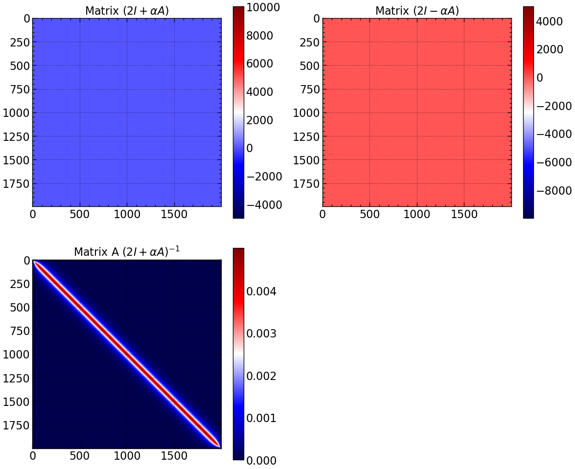
for which \(T\) is a \(N-2 \times N-2\) matrix:
\(S\) is another \(N-2 \times N-2\) matrix:
\(\mathbf{B}_j\) is a column vector of size N-2 containing \(B_{ij}\) values, \(\mathbf{b}_j\) and \(\mathbf{b}_{j+1}\) are column vectors of size N-2 representing the boundary conditions for the current and next time steps, respectively.
#  A and B
A = np.zeros((N-1, N-1))
B = np.zeros((N-1, N-1))
for i in range(N-1):
    A[i, i] = 2 + 2 * r
    B[i, i] = 2 - 2 * r
    if i < N-2:
        A[i, i+1] = -r
        A[i+1, i] = -r
        B[i, i+1] = r
        B[i+1, i] = r

# inverse of A
A_inv = np.linalg.inv(A)

fig, axs = plt.subplots(2, 2, figsize=(12, 10))
im = axs[0, 0].imshow(A, cmap='seismic')
axs[0, 0].set_title(r'Matrix $(2I + \alpha A)$')
plt.colorbar(im, ax=axs[0, 0])
im = axs[0, 1].imshow(B, cmap='seismic')
axs[0, 1].set_title(r'Matrix $(2I - \alpha A)$')
plt.colorbar(im, ax=axs[0, 1])
im = axs[1, 0].imshow(A_inv, cmap='seismic')
axs[1, 0].set_title(r'Matrix A $(2I + \alpha A)^{-1}$')
plt.colorbar(im, ax=axs[1, 0])
axs[1, 1].axis('off')

plt.tight_layout()
plt.savefig("seed_1/matrix_A_B_A_inv.pdf")
plt.show()
for j in range (1,time_steps+1):
    b1[0]=r*Br[0,j-1]+r*Br[0,j]
    b1[N-2]=r*Br[N,j-1]+r*Br[N,j]
    v1=np.dot(B,Br[1:(N),j-1])
    Br[1:(N),j]=np.dot(A_inv,v1+b1)

    b2[0]=r*Bphi[0,j-1]+r*Bphi[0,j]
    b2[N-2]=r*Bphi[N,j-1]+r*Bphi[N,j]
    v2=np.dot(B,Bphi[1:(N),j-1])
    Bphi[1:(N),j]=np.dot(A_inv,v2+b2)
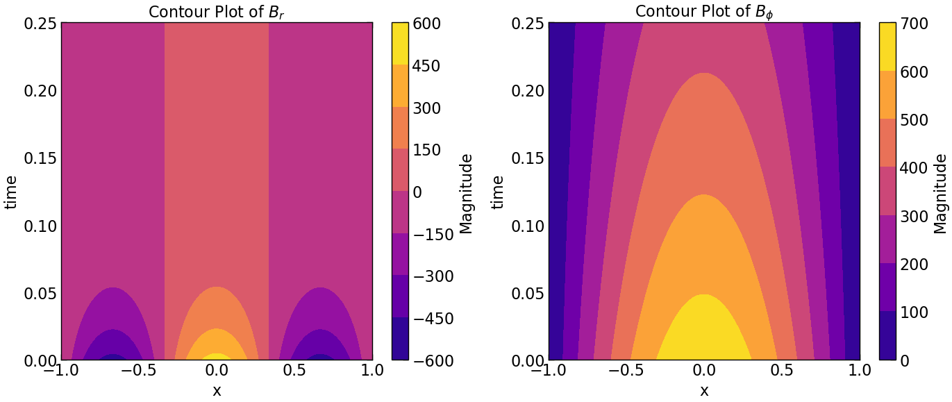
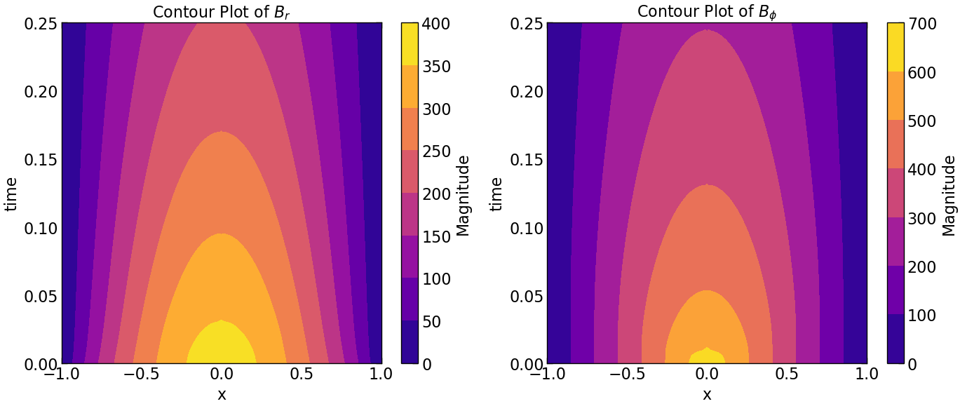
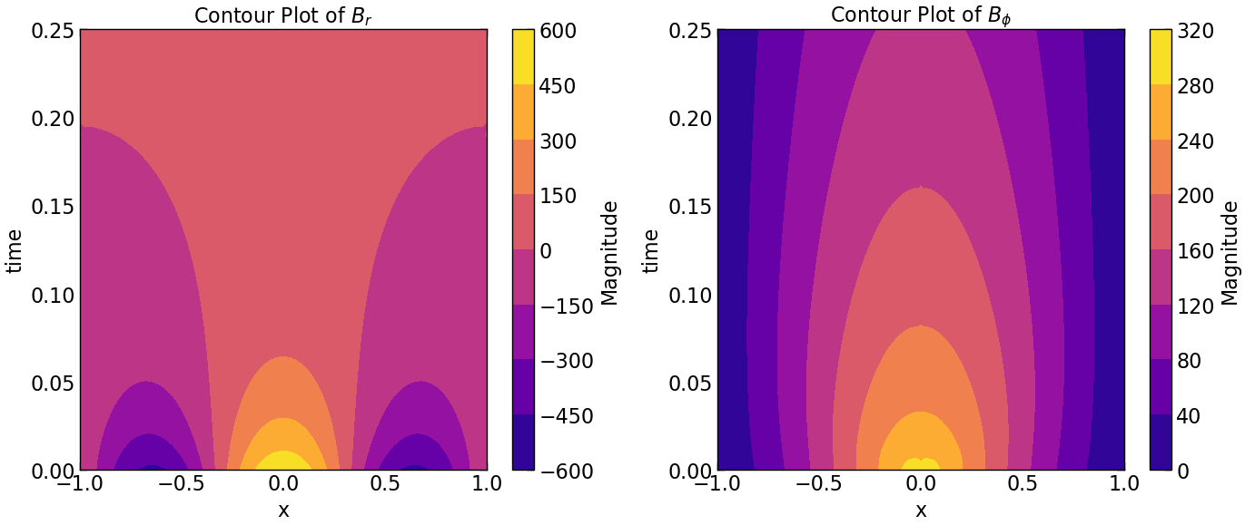
plt.figure(figsize=(14, 6))

plt.subplot(1, 2, 1)
plt.contourf(Z, Y, Br.transpose(), cmap='plasma')
plt.colorbar(label='Magnitude')
plt.xlabel('x')
plt.ylabel('time')
plt.title(r'Contour Plot of $B_r$')

plt.subplot(1, 2, 2)
plt.contourf(Z, Y, Bphi.transpose(), cmap='plasma')
plt.colorbar(label='Magnitude')
plt.xlabel('x')
plt.ylabel('time')
plt.title(r'Contour Plot of $B_{\phi}$')

plt.tight_layout()
plt.savefig("seed_1/contour_plot_Br_Bphi.pdf")
plt.show()
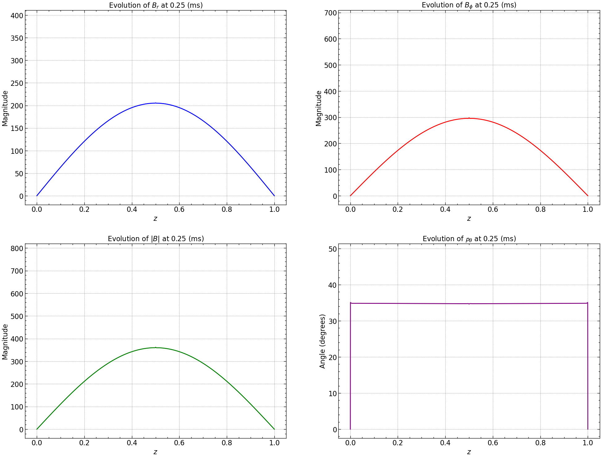
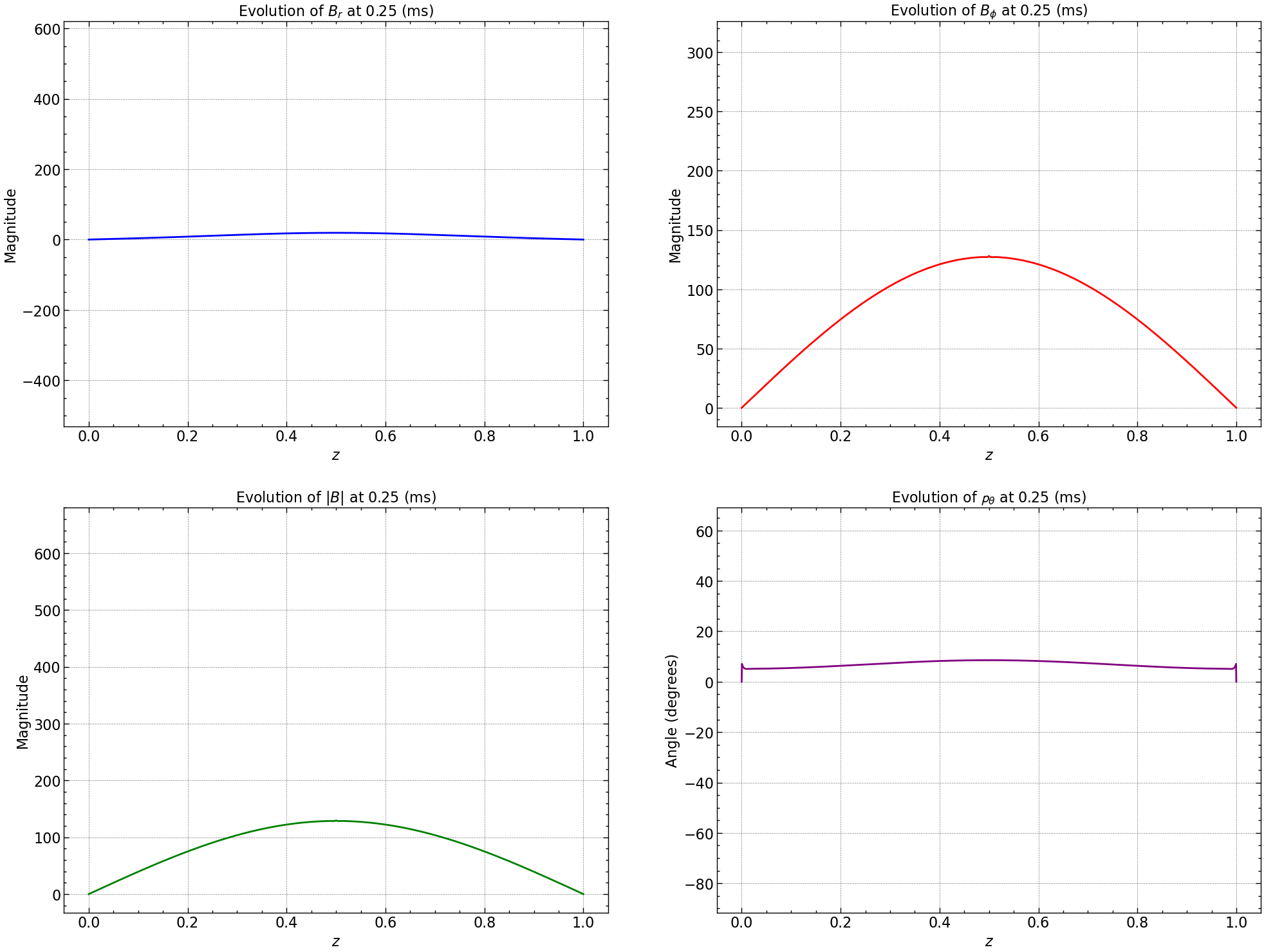
norm_squared_sum = np.sqrt(Br**2 + Bphi**2)
pitch_angle = np.arctan2(Br, Bphi) * (180 / np.pi)
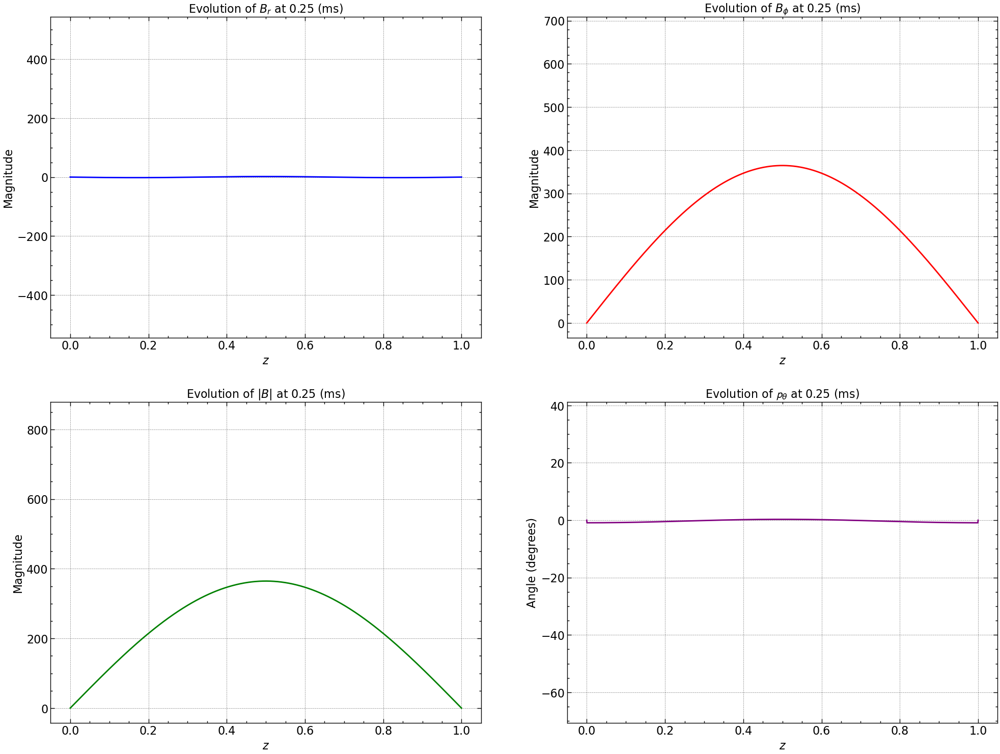
fig, axs = plt.subplots(2, 2, figsize=(24, 18))
# Plot Br
line_br, = axs[0, 0].plot(np.linspace(0, 1, Br.shape[0]), Br[:, 0], color='blue', label='Br')
axs[0, 0].set_xlabel(r'$z$')
axs[0, 0].set_ylabel('Magnitude')
axs[0, 0].set_title(r'Evolution of $B_r$')
# Plot Bphi
line_bphi, = axs[0, 1].plot(np.linspace(0, 1, Bphi.shape[0]), Bphi[:, 0], color='red', label='Bphi')
axs[0, 1].set_xlabel(r'$z$')
axs[0, 1].set_ylabel('Magnitude')
axs[0, 1].set_title(r'Evolution of $B_{\phi}$')
# Plot Norm
line_norm, = axs[1, 0].plot(np.linspace(0, 1, norm_squared_sum.shape[0]), norm_squared_sum[:, 0], color='green', label='Norm')
axs[1, 0].set_xlabel(r'$z$')
axs[1, 0].set_ylabel('Magnitude')
axs[1, 0].set_title(r'Evolution of $|B|$')
line_pitch, = axs[1, 1].plot(np.linspace(0, 1, pitch_angle.shape[0]), pitch_angle[:, 0], color='purple', label='Pitch Angle')
axs[1, 1].set_xlabel(r'$z$')
axs[1, 1].set_ylabel('Angle (degrees)')
axs[1, 1].set_title(r'Evolution of Pitch Angle ($\mathbf{p}_{\theta}$)')
def update(frame):
time = frame * k
line_br.set_ydata(Br[:, frame])
axs[0, 0].set_title(r'Evolution of $B_r$ at %s (ms)' % time)
line_bphi.set_ydata(Bphi[:, frame])
axs[0, 1].set_title(r'Evolution of $B_{\phi}$ at %s (ms)' % time)
line_norm.set_ydata(norm_squared_sum[:, frame])
axs[1, 0].set_title(r'Evolution of $|B|$ at %s (ms)' % time)
line_pitch.set_ydata(pitch_angle[:, frame])
axs[1, 1].set_title(r'Evolution of $\mathcal{p}_{\theta}$ at %s (ms)' % time)
return line_br, line_bphi, line_norm, line_pitch
ani = FuncAnimation(fig, update, frames=range(Br.shape[1]), interval=100)
ani.save('seed_1/Br_Bphi_Norm_Pitch_evolution.gif', writer='pillow')
plt.show()
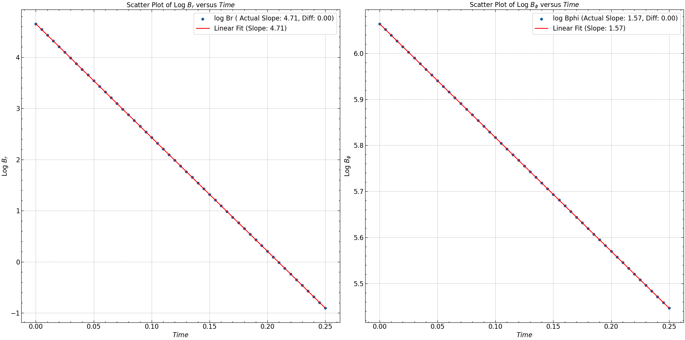
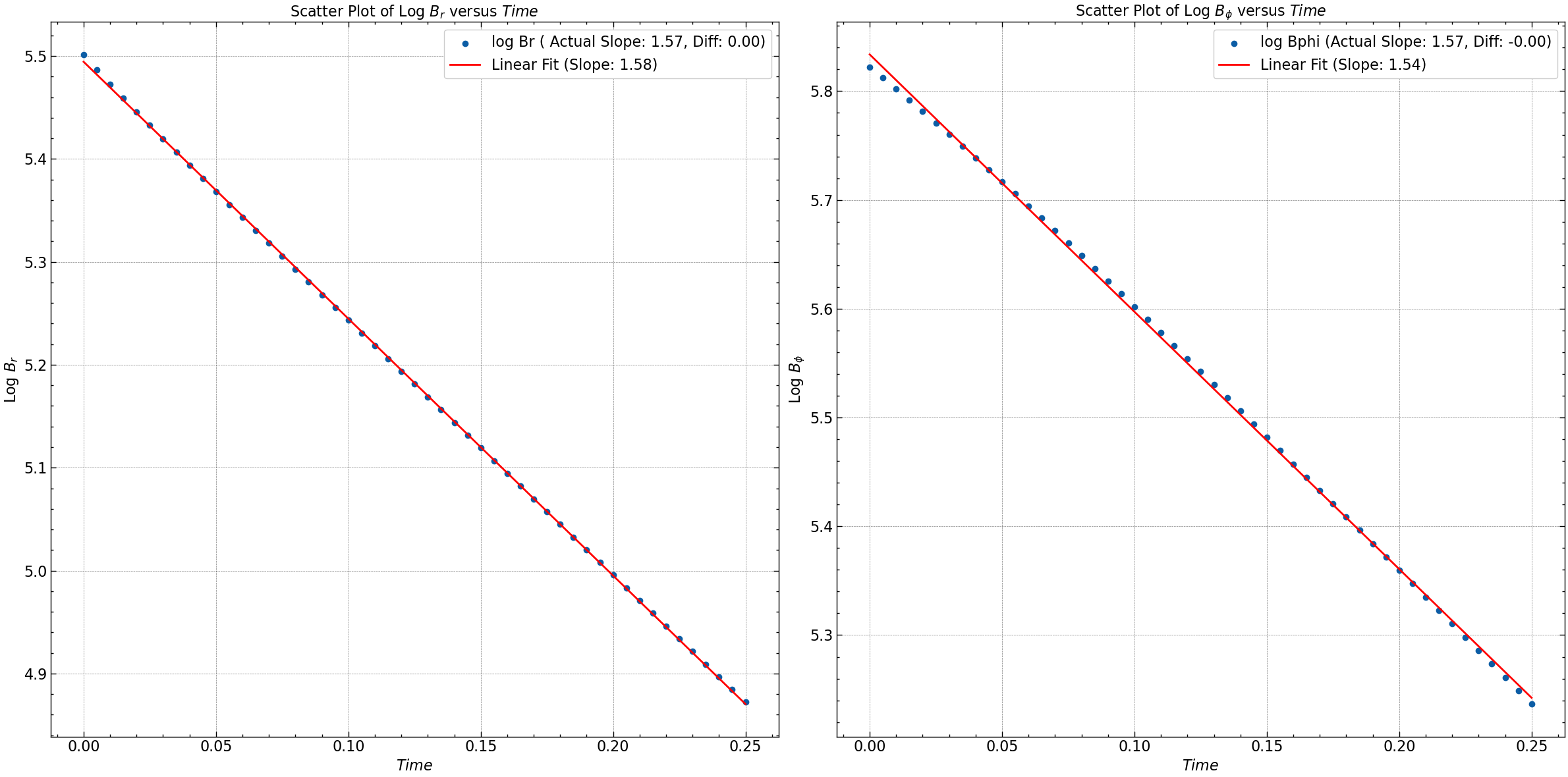
log_Br = np.log(np.abs(Br.mean(axis=0)))
log_Bphi = np.log(np.abs(Bphi.mean(axis=0)))

slope_Br, intercept_Br = np.polyfit(time, log_Br, 1)
slope_Bphi, intercept_Bphi = np.polyfit(time, log_Bphi, 1)

actual_slope_Br = (m + 1/2)* np.pi
actual_slope_Bphi = (n + 1/2)* np.pi

difference_Br = np.sqrt(-slope_Br) - actual_slope_Br
difference_Bphi = np.sqrt(-slope_Bphi) - actual_slope_Bphi

print(f"Br: Actual Slope = {actual_slope_Br}, Computed Slope = {np.sqrt(-slope_Br)}, Difference = {difference_Br}")
print(f"Bphi: Actual Slope = {actual_slope_Bphi}, Computed Slope = {np.sqrt(-slope_Bphi)}, Difference = {difference_Bphi}")
Br: Actual Slope = 4.71238898038469, Computed Slope = 4.714809134907199, Difference = 0.0024201545225093213
Bphi: Actual Slope = 1.5707963267948966, Computed Slope = 1.5708061270906244, Difference = 9.800295727835362e-06
plt.figure(figsize=(24, 12))

# Scatter plot for log Br
plt.subplot(1, 2, 1)
plt.scatter(time, log_Br, label=f'log Br ( Actual Slope: {actual_slope_Br:.2f}, Diff: {difference_Br:.2f})')
plt.xlabel(r'$Time$')
plt.ylabel(r'Log $B_r$')
plt.title(r'Scatter Plot of Log $B_r$ versus $Time$')
plt.grid(True)

# Linear fit for log Br
fit_Br = np.polyfit(time, log_Br, 1)
plt.plot(time, np.polyval(fit_Br, time), color='red', label=f'Linear Fit (Slope: {np.sqrt(-fit_Br[0]):.2f})')
plt.legend()

# Scatter plot for log Bphi
plt.subplot(1, 2, 2)
plt.scatter(time, log_Bphi, label=f'log Bphi (Actual Slope: {actual_slope_Bphi:.2f}, Diff: {difference_Bphi:.2f})')
plt.xlabel(r'$Time$')
plt.ylabel(r'Log $B_{\phi}$')
plt.title(r'Scatter Plot of Log $B_{\phi}$ versus $Time$')
plt.grid(True)

# Linear fit for log Bphi
fit_Bphi = np.polyfit(time, log_Bphi, 1)
plt.plot(time, np.polyval(fit_Bphi, time), color='red', label=f'Linear Fit (Slope: {np.sqrt(-fit_Bphi[0]):.2f})')
plt.legend()

plt.tight_layout()
plt.savefig("seed_1/log_Br_Bphi_vs_time.png")
plt.show()
Seed 2: Exponential Decay Solution
def generate_random_Bo(seed_value):
    np.random.seed(seed_value)
    random_float = np.random.rand()
    return random_float

def initial_conditions(N, time_steps, seed_value, gamma, BCtype = "vacuum"):
    mag_br = 1000*generate_random_Bo(seed_value)
    mag_bphi = 1000*generate_random_Bo(seed_value + 1)

    z = np.linspace(-1, 1, N+1)
    Br = np.zeros((N+1, time_steps+1))
    Bphi = np.zeros((N+1, time_steps+1))
    b1 = np.zeros(N-1)
    b2 = np.zeros(N-1)

    # Initial Condition for Br and Bphi
    for i in range(1, N+1):
        Br[i, 0] = mag_br * (1 - np.exp( -gamma * (1-np.abs(z[i]))))
        Bphi[i, 0] = mag_bphi * (1 - np.abs(z[i]))

    # Boundary Condition
    if BCtype == "vacuum":
        Br[0, :] = 0
        Bphi[0, :] = 0
        Br[N, :] = 0
        Bphi[N, :] = 0

    return z, Br, Bphi, b1, b2, mag_br, mag_bphi
seed_value = 50
gamma = np.pi/2
z, Br, Bphi, b1, b2, mag_br, mag_bphi = initial_conditions(N, time_steps, seed_value, gamma)
fig, axs = plt.subplots(2, figsize=(15, 20))

axs[0].plot(z, Br[:, 0], label=f'Initial Condition (Br, mag={mag_br:.2f})', color='blue')
axs[0].plot(z, Bphi[:,0], label=f'Initial Condition (Bphi, mag={mag_bphi:.2f})', color='orange')
axs[0].plot(z[[0, N]], Br[[0, N], 0], 'go', markersize=8, label='Boundary Condition at t[0]=0')
axs[0].set_title(r'Initial Conditions for $B_{r}$ and $B_{\phi}$', fontsize=18)
axs[0].set_xlabel(r'$z$', fontsize=14)
axs[0].set_ylabel('Magnitude', fontsize=14)
axs[0].legend(loc='upper right', fontsize=12)
axs[0].grid(True, linestyle='--', alpha=0.5)


norm_Br_Bphi = [np.linalg.norm(np.sqrt(Br[i, 0]**2 + Bphi[:,0]**2)) for i in range(len(z))]
axs[1].plot(z, norm_Br_Bphi , label=r'Norm of ($B_r$, $B_{\phi}$)', linestyle='-', color='red')
axs[1].set_title(r'Norm of ($B_{r}$, $B_{\phi}$)', fontsize=18)
axs[1].set_xlabel(r'$z$', fontsize=14)
axs[1].set_ylabel('Magnitude', fontsize=14)
axs[1].legend(loc='upper right', fontsize=12)
axs[1].grid(True, linestyle='--', alpha=0.5)

plt.tight_layout()
plt.savefig("seed_2/initial_conditions.pdf")
plt.show()
#  A and B
A = np.zeros((N-1, N-1))
B = np.zeros((N-1, N-1))
for i in range(N-1):
    A[i, i] = 2 + 2 * r
    B[i, i] = 2 - 2 * r
    if i < N-2:
        A[i, i+1] = -r
        A[i+1, i] = -r
        B[i, i+1] = r
        B[i+1, i] = r

# inverse of A
A_inv = np.linalg.inv(A)

fig, axs = plt.subplots(2, 2, figsize=(12, 10))
im = axs[0, 0].imshow(A, cmap='seismic')
axs[0, 0].set_title(r'Matrix $(2I + \alpha A)$')
plt.colorbar(im, ax=axs[0, 0])
im = axs[0, 1].imshow(B, cmap='seismic')
axs[0, 1].set_title(r'Matrix $(2I - \alpha A)$')
plt.colorbar(im, ax=axs[0, 1])
im = axs[1, 0].imshow(A_inv, cmap='seismic')
axs[1, 0].set_title(r'Matrix A $(2I + \alpha A)^{-1}$')
plt.colorbar(im, ax=axs[1, 0])
axs[1, 1].axis('off')

plt.tight_layout()
plt.savefig("seed_2/matrix_A_B_A_inv.pdf")
plt.show()
for j in range (1,time_steps+1):
    b1[0]=r*Br[0,j-1]+r*Br[0,j]
    b1[N-2]=r*Br[N,j-1]+r*Br[N,j]
    v1=np.dot(B,Br[1:(N),j-1])
    Br[1:(N),j]=np.dot(A_inv,v1+b1)

    b2[0]=r*Bphi[0,j-1]+r*Bphi[0,j]
    b2[N-2]=r*Bphi[N,j-1]+r*Bphi[N,j]
    v2=np.dot(B,Bphi[1:(N),j-1])
    Bphi[1:(N),j]=np.dot(A_inv,v2+b2)
plt.figure(figsize=(14, 6))

plt.subplot(1, 2, 1)
plt.contourf(Z, Y, Br.transpose(), cmap='plasma')
plt.colorbar(label='Magnitude')
plt.xlabel('x')
plt.ylabel('time')
plt.title(r'Contour Plot of $B_r$')

plt.subplot(1, 2, 2)
plt.contourf(Z, Y, Bphi.transpose(), cmap='plasma')
plt.colorbar(label='Magnitude')
plt.xlabel('x')
plt.ylabel('time')
plt.title(r'Contour Plot of $B_{\phi}$')

plt.tight_layout()
plt.savefig("seed_2/contour_plot_Br_Bphi.pdf")
plt.show()
norm_squared_sum = np.sqrt(Br**2 + Bphi**2)
pitch_angle = np.arctan2(Br, Bphi) * (180 / np.pi)

fig, axs = plt.subplots(2, 2, figsize=(24, 18))
# Plot Br
line_br, = axs[0, 0].plot(np.linspace(0, 1, Br.shape[0]), Br[:, 0], color='blue', label='Br')
axs[0, 0].set_xlabel(r'$z$')
axs[0, 0].set_ylabel('Magnitude')
axs[0, 0].set_title(r'Evolution of $B_r$')

# Plot Bphi
line_bphi, = axs[0, 1].plot(np.linspace(0, 1, Bphi.shape[0]), Bphi[:, 0], color='red', label='Bphi')
axs[0, 1].set_xlabel(r'$z$')
axs[0, 1].set_ylabel('Magnitude')
axs[0, 1].set_title(r'Evolution of $B_{\phi}$')

# Plot Norm
line_norm, = axs[1, 0].plot(np.linspace(0, 1, norm_squared_sum.shape[0]), norm_squared_sum[:, 0], color='green', label='Norm')
axs[1, 0].set_xlabel(r'$z$')
axs[1, 0].set_ylabel('Magnitude')
axs[1, 0].set_title(r'Evolution of $|B|$')


line_pitch, = axs[1, 1].plot(np.linspace(0, 1, pitch_angle.shape[0]), pitch_angle[:, 0], color='purple', label='Pitch Angle')
axs[1, 1].set_xlabel(r'$z$')
axs[1, 1].set_ylabel('Angle (degrees)')
axs[1, 1].set_title(r'Evolution of Pitch Angle ($\mathbf{p}_{\theta}$)')

def update(frame):
    time = frame * k
    line_br.set_ydata(Br[:, frame])
    axs[0, 0].set_title(r'Evolution of $B_r$ at %s (ms)' % time)

    line_bphi.set_ydata(Bphi[:, frame])
    axs[0, 1].set_title(r'Evolution of $B_{\phi}$ at %s (ms)' % time)

    line_norm.set_ydata(norm_squared_sum[:, frame])
    axs[1, 0].set_title(r'Evolution of $|B|$ at %s (ms)' % time)

    line_pitch.set_ydata(pitch_angle[:, frame])
    axs[1, 1].set_title(r'Evolution of $\mathcal{p}_{\theta}$ at %s (ms)' % time)

    return line_br, line_bphi, line_norm, line_pitch

ani = FuncAnimation(fig, update, frames=range(Br.shape[1]), interval=100)
ani.save('seed_2/Br_Bphi_Norm_Pitch_evolution.gif', writer='pillow')

plt.show()
log_Br = np.log(np.abs(Br.mean(axis=0)))
log_Bphi = np.log(np.abs(Bphi.mean(axis=0)))

slope_Br, intercept_Br = np.polyfit(time[-20:], log_Br[-20:], 1)
slope_Bphi, intercept_Bphi = np.polyfit(time[-20:], log_Bphi[-20:], 1)

actual_slope_Br = gamma
actual_slope_Bphi = gamma

difference_Br = np.sqrt(-slope_Br) - actual_slope_Br
difference_Bphi = np.sqrt(-slope_Bphi) - actual_slope_Bphi

print(f"Br: Actual Slope = {actual_slope_Br}, Computed Slope = {np.sqrt(-slope_Br)}, Difference = {difference_Br}")
print(f"Bphi: Actual Slope = {actual_slope_Bphi}, Computed Slope = {np.sqrt(-slope_Bphi)}, Difference = {difference_Bphi}")
Br: Actual Slope = 1.5707963267948966, Computed Slope = 1.571682875158095, Difference = 0.0008865483631983473
Bphi: Actual Slope = 1.5707963267948966, Computed Slope = 1.5661093922713243, Difference = -0.004686934523572273
plt.figure(figsize=(24, 12))

# Scatter plot for log Br
plt.subplot(1, 2, 1)
plt.scatter(time, log_Br, label=f'log Br ( Actual Slope: {actual_slope_Br:.2f}, Diff: {difference_Br:.2f})')
plt.xlabel(r'$Time$')
plt.ylabel(r'Log $B_r$')
plt.title(r'Scatter Plot of Log $B_r$ versus $Time$')
plt.grid(True)

# Linear fit for log Br
fit_Br = np.polyfit(time, log_Br, 1)
plt.plot(time, np.polyval(fit_Br, time), color='red', label=f'Linear Fit (Slope: {np.sqrt(-fit_Br[0]):.2f})')
plt.legend()

# Scatter plot for log Bphi
plt.subplot(1, 2, 2)
plt.scatter(time, log_Bphi, label=f'log Bphi (Actual Slope: {actual_slope_Bphi:.2f}, Diff: {difference_Bphi:.2f})')
plt.xlabel(r'$Time$')
plt.ylabel(r'Log $B_{\phi}$')
plt.title(r'Scatter Plot of Log $B_{\phi}$ versus $Time$')
plt.grid(True)

# Linear fit for log Bphi
fit_Bphi = np.polyfit(time, log_Bphi, 1)
plt.plot(time, np.polyval(fit_Bphi, time), color='red', label=f'Linear Fit (Slope: {np.sqrt(-fit_Bphi[0]):.2f})')
plt.legend()

plt.tight_layout()
plt.savefig("seed_2/log_Br_Bphi_vs_time.png")
plt.show()
Seed 3: Gaussian & Trigonometric Decay Solution
def generate_random_Bo(seed_value):
    np.random.seed(seed_value)
    random_float = np.random.rand()
    return random_float

def initial_conditions(N, time_steps, seed_value, sigma, BCtype = "vacuum"):
    mag_br = 1000*generate_random_Bo(seed_value)
    mag_bphi = 1000*generate_random_Bo(seed_value + 1)

    z = np.linspace(-1, 1, N+1)
    Br = np.zeros((N+1, time_steps+1))
    Bphi = np.zeros((N+1, time_steps+1))
    b1 = np.zeros(N-1)
    b2 = np.zeros(N-1)

    # Initial Condition for Br and Bphi
    for i in range(1, N+1):
        Br[i, 0] = mag_br * np.exp( - z[i]**2/sigma**2) * np.cos(3*np.pi/2 * z[i])
        Bphi[i, 0] = mag_bphi * np.exp(- np.abs(z[i])) * np.cos(np.pi/2 * z[i])

    # Boundary Condition
    if BCtype == "vacuum":
        Br[0, :] = 0
        Bphi[0, :] = 0
        Br[N, :] = 0
        Bphi[N, :] = 0

    return z, Br, Bphi, b1, b2, mag_br, mag_bphi
seed_value = 75
sigma = np.pi/2
z, Br, Bphi, b1, b2, mag_br, mag_bphi = initial_conditions(N, time_steps, seed_value, sigma)
fig, axs = plt.subplots(2, figsize=(15, 20))

axs[0].plot(z, Br[:, 0], label=f'Initial Condition (Br, mag={mag_br:.2f})', color='blue')
axs[0].plot(z, Bphi[:,0], label=f'Initial Condition (Bphi, mag={mag_bphi:.2f})', color='orange')
axs[0].plot(z[[0, N]], Br[[0, N], 0], 'go', markersize=8, label='Boundary Condition at t[0]=0')
axs[0].set_title(r'Initial Conditions for $B_{r}$ and $B_{\phi}$', fontsize=18)
axs[0].set_xlabel(r'$z$', fontsize=14)
axs[0].set_ylabel('Magnitude', fontsize=14)
axs[0].legend(loc='upper right', fontsize=12)
axs[0].grid(True, linestyle='--', alpha=0.5)


norm_Br_Bphi = [np.linalg.norm(np.sqrt(Br[i, 0]**2 + Bphi[:,0]**2)) for i in range(len(z))]
axs[1].plot(z, norm_Br_Bphi , label=r'Norm of ($B_r$, $B_{\phi}$)', linestyle='-', color='red')
axs[1].set_title(r'Norm of ($B_{r}$, $B_{\phi}$)', fontsize=18)
axs[1].set_xlabel(r'$z$', fontsize=14)
axs[1].set_ylabel('Magnitude', fontsize=14)
axs[1].legend(loc='upper right', fontsize=12)
axs[1].grid(True, linestyle='--', alpha=0.5)

plt.tight_layout()
plt.savefig("seed_3/initial_conditions.pdf")
plt.show()
#  A and B
A = np.zeros((N-1, N-1))
B = np.zeros((N-1, N-1))
for i in range(N-1):
    A[i, i] = 2 + 2 * r
    B[i, i] = 2 - 2 * r
    if i < N-2:
        A[i, i+1] = -r
        A[i+1, i] = -r
        B[i, i+1] = r
        B[i+1, i] = r

# inverse of A
A_inv = np.linalg.inv(A)

fig, axs = plt.subplots(2, 2, figsize=(12, 10))
im = axs[0, 0].imshow(A, cmap='seismic')
axs[0, 0].set_title(r'Matrix $(2I + \alpha A)$')
plt.colorbar(im, ax=axs[0, 0])
im = axs[0, 1].imshow(B, cmap='seismic')
axs[0, 1].set_title(r'Matrix $(2I - \alpha A)$')
plt.colorbar(im, ax=axs[0, 1])
im = axs[1, 0].imshow(A_inv, cmap='seismic')
axs[1, 0].set_title(r'Matrix A $(2I + \alpha A)^{-1}$')
plt.colorbar(im, ax=axs[1, 0])
axs[1, 1].axis('off')

plt.tight_layout()
plt.savefig("seed_3/matrix_A_B_A_inv.pdf")
plt.show()
for j in range (1,time_steps+1):
    b1[0]=r*Br[0,j-1]+r*Br[0,j]
    b1[N-2]=r*Br[N,j-1]+r*Br[N,j]
    v1=np.dot(B,Br[1:(N),j-1])
    Br[1:(N),j]=np.dot(A_inv,v1+b1)

    b2[0]=r*Bphi[0,j-1]+r*Bphi[0,j]
    b2[N-2]=r*Bphi[N,j-1]+r*Bphi[N,j]
    v2=np.dot(B,Bphi[1:(N),j-1])
    Bphi[1:(N),j]=np.dot(A_inv,v2+b2)
plt.figure(figsize=(14, 6))

plt.subplot(1, 2, 1)
plt.contourf(Z, Y, Br.transpose(), cmap='plasma')
plt.colorbar(label='Magnitude')
plt.xlabel('x')
plt.ylabel('time')
plt.title(r'Contour Plot of $B_r$')

plt.subplot(1, 2, 2)
plt.contourf(Z, Y, Bphi.transpose(), cmap='plasma')
plt.colorbar(label='Magnitude')
plt.xlabel('x')
plt.ylabel('time')
plt.title(r'Contour Plot of $B_{\phi}$')

plt.tight_layout()
plt.savefig("seed_3/contour_plot_Br_Bphi.pdf")
plt.show()
norm_squared_sum = np.sqrt(Br**2 + Bphi**2)
pitch_angle = np.arctan2(Br, Bphi) * (180 / np.pi)

fig, axs = plt.subplots(2, 2, figsize=(24, 18))
# Plot Br
line_br, = axs[0, 0].plot(np.linspace(0, 1, Br.shape[0]), Br[:, 0], color='blue', label='Br')
axs[0, 0].set_xlabel(r'$z$')
axs[0, 0].set_ylabel('Magnitude')
axs[0, 0].set_title(r'Evolution of $B_r$')

# Plot Bphi
line_bphi, = axs[0, 1].plot(np.linspace(0, 1, Bphi.shape[0]), Bphi[:, 0], color='red', label='Bphi')
axs[0, 1].set_xlabel(r'$z$')
axs[0, 1].set_ylabel('Magnitude')
axs[0, 1].set_title(r'Evolution of $B_{\phi}$')

# Plot Norm
line_norm, = axs[1, 0].plot(np.linspace(0, 1, norm_squared_sum.shape[0]), norm_squared_sum[:, 0], color='green', label='Norm')
axs[1, 0].set_xlabel(r'$z$')
axs[1, 0].set_ylabel('Magnitude')
axs[1, 0].set_title(r'Evolution of $|B|$')


line_pitch, = axs[1, 1].plot(np.linspace(0, 1, pitch_angle.shape[0]), pitch_angle[:, 0], color='purple', label='Pitch Angle')
axs[1, 1].set_xlabel(r'$z$')
axs[1, 1].set_ylabel('Angle (degrees)')
axs[1, 1].set_title(r'Evolution of Pitch Angle ($\mathbf{p}_{\theta}$)')

def update(frame):
    time = frame * k
    line_br.set_ydata(Br[:, frame])
    axs[0, 0].set_title(r'Evolution of $B_r$ at %s (ms)' % time)

    line_bphi.set_ydata(Bphi[:, frame])
    axs[0, 1].set_title(r'Evolution of $B_{\phi}$ at %s (ms)' % time)

    line_norm.set_ydata(norm_squared_sum[:, frame])
    axs[1, 0].set_title(r'Evolution of $|B|$ at %s (ms)' % time)

    line_pitch.set_ydata(pitch_angle[:, frame])
    axs[1, 1].set_title(r'Evolution of $\mathcal{p}_{\theta}$ at %s (ms)' % time)

    return line_br, line_bphi, line_norm, line_pitch

ani = FuncAnimation(fig, update, frames=range(Br.shape[1]), interval=100)
ani.save('seed_3/Br_Bphi_Norm_Pitch_evolution.gif', writer='pillow')

plt.show()
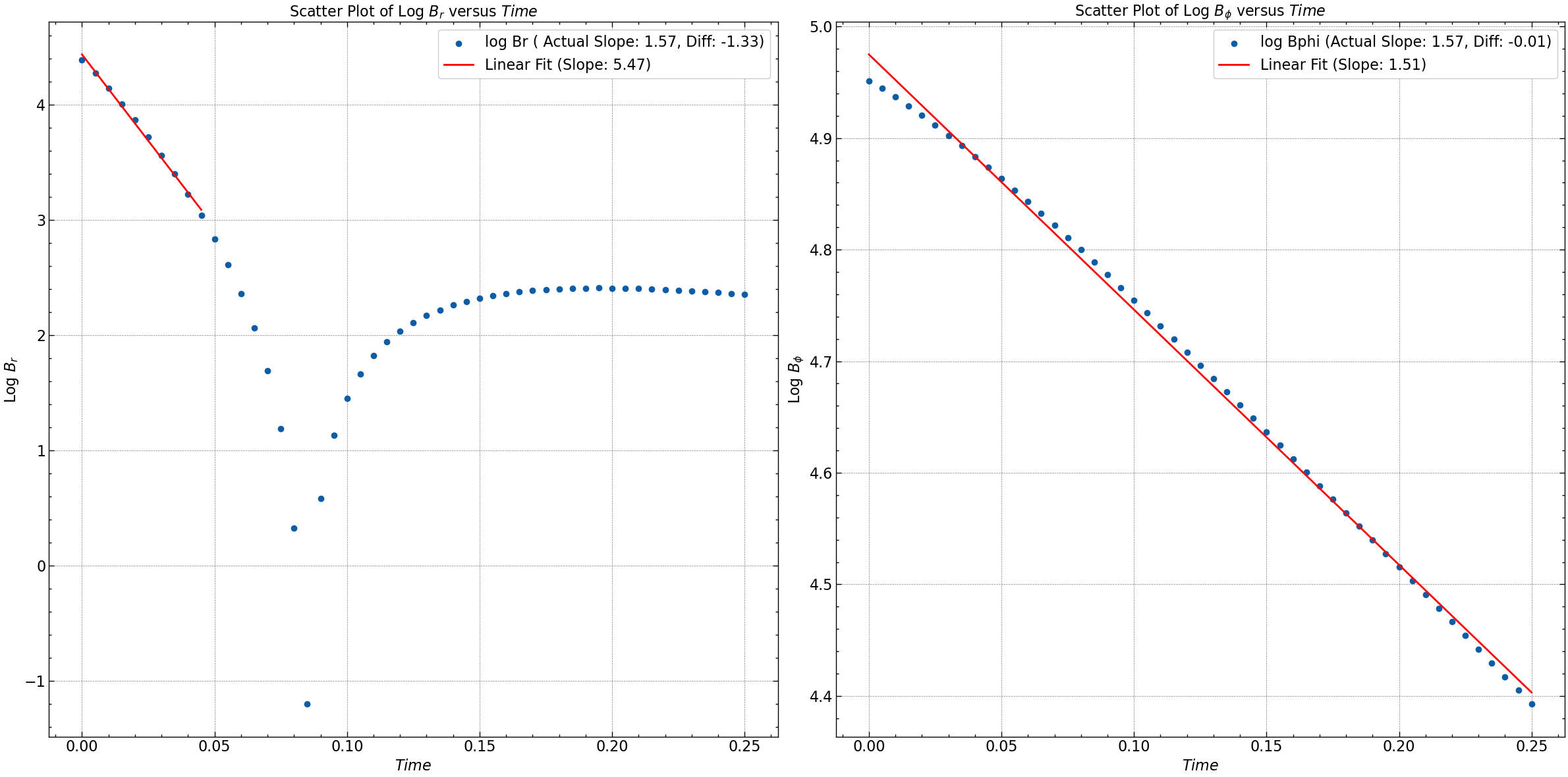
log_Br = np.log(np.abs(Br.mean(axis=0)))
log_Bphi = np.log(np.abs(Bphi.mean(axis=0)))

slope_Br, intercept_Br = np.polyfit(time[-20:], log_Br[-20:], 1)
slope_Bphi, intercept_Bphi = np.polyfit(time[-20:], log_Bphi[-20:], 1)

actual_slope_Br = sigma
actual_slope_Bphi = sigma

difference_Br = np.sqrt(-slope_Br) - actual_slope_Br
difference_Bphi = np.sqrt(-slope_Bphi) - actual_slope_Bphi

print(f"Br: Actual Slope = {actual_slope_Br}, Computed Slope = {np.sqrt(-slope_Br)}, Difference = {difference_Br}")
print(f"Bphi: Actual Slope = {actual_slope_Bphi}, Computed Slope = {np.sqrt(-slope_Bphi)}, Difference = {difference_Bphi}")
Br: Actual Slope = 1.5707963267948966, Computed Slope = 0.241748758558783, Difference = -1.3290475682361136
Bphi: Actual Slope = 1.5707963267948966, Computed Slope = 1.5629031592116118, Difference = -0.007893167583284733
plt.figure(figsize=(24, 12))

# Scatter plot for log Br
plt.subplot(1, 2, 1)
plt.scatter(time, log_Br, label=f'log Br ( Actual Slope: {actual_slope_Br:.2f}, Diff: {difference_Br:.2f})')
plt.xlabel(r'$Time$')
plt.ylabel(r'Log $B_r$')
plt.title(r'Scatter Plot of Log $B_r$ versus $Time$')
plt.grid(True)

# Linear fit for log Br
fit_Br = np.polyfit(time[:10], log_Br[:10], 1)
plt.plot(time[:10], np.polyval(fit_Br[:10], time[:10]), color='red', label=f'Linear Fit (Slope: {np.sqrt(-fit_Br[0]):.2f})')
plt.legend()

# Scatter plot for log Bphi
plt.subplot(1, 2, 2)
plt.scatter(time, log_Bphi, label=f'log Bphi (Actual Slope: {actual_slope_Bphi:.2f}, Diff: {difference_Bphi:.2f})')
plt.xlabel(r'$Time$')
plt.ylabel(r'Log $B_{\phi}$')
plt.title(r'Scatter Plot of Log $B_{\phi}$ versus $Time$')
plt.grid(True)

# Linear fit for log Bphi
fit_Bphi = np.polyfit(time, log_Bphi, 1)
plt.plot(time, np.polyval(fit_Bphi, time), color='red', label=f'Linear Fit (Slope: {np.sqrt(-fit_Bphi[0]):.2f})')
plt.legend()

plt.tight_layout()
plt.savefig("seed_3/log_Br_Bphi_vs_time.png")
plt.show()