Solving Galactic Diffusion Equation using Crank Nicholson (W/ Ghost Zones)

Solving Galactic Diffusion Equation using Crank Nicholson (W/ Ghost Zones)#

This notebook will illustrate the crank nicholson difference method solving Galactic Dynamo Diffusion Equation.

The implicit Crank-Nicolson difference equation of the Dynamo equation is derived by discretizing the following coupled equations

\[ \frac{\partial \bar{B}_r}{\partial t} = \eta_t\frac{\partial^2 \bar{B}_r}{\partial z^2} \]

\[ \frac{\partial \bar{B}_\phi}{\partial t} = \eta_t \frac{\partial^2 \bar{B}_\phi}{\partial z^2} \]

Where $\eta_t$ is currently constant parameter called the magnetic diffusivity.

import numpy as np
import tabulate
from PIL import Image

import matplotlib.pyplot as plt 
import scienceplots
plt.style.use(['science', 'notebook', 'grid']) 
from matplotlib.animation import FuncAnimation
from IPython import display

from matplotlib import rcParams
rcParams['axes.grid'] = True
rcParams['grid.linestyle'] = '--'
rcParams['grid.alpha'] = 0.5
%matplotlib inline

import warnings
warnings.filterwarnings("ignore")

Discrete Grid#

Spatial Discretization:

We divide the spatial domain $z$ into $N$ grid points. Let $h$ denote the spacing between consecutive grid points.
Time Discretization:

We discretize the time domain $t$ into time steps of size $k$.

The region $\Omega$ is discretised into a uniform mesh $\Omega_h$. In the space $x$ direction into $N$ steps giving a stepsize of

\[ h=\frac{1-0}{N} \]

resulting in

\[ x[i]=0+ih, \ \ \ i=0,1,...,N, \]

and into $N_t$ steps in the time $t$ direction giving a stepsize of

\[ k=\frac{1-0}{N_t} \]

resulting in

\[ t[i]=0+ik, \ \ \ k=0,...,K.\]

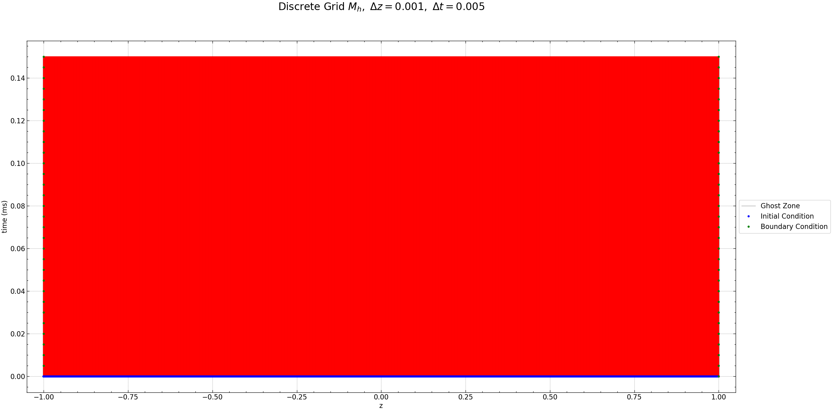
The Figure below shows the discrete grid points for $N$ space points and $N_t$ time points , the red dots are the unknown values, the green dots are the known boundary conditions and the blue dots are the known initial conditions of the diffusion Equation. Additionally, ghost zones are included at the first and last indices. These ghost zones are crucial for defining derivatives at the boundary.

Ghost Zones#

Ghost zones are introduced to extend the computational domain slightly beyond the physical domain. They essentially serve as buffer zones at the boundaries, enabling the application of boundary conditions and accurate computation of derivatives.

Seed 1: Oscillatory Solution

\[ B_r = B_o \cdot sin(2 \pi z) \]

\[ B_r = B_o \cdot sin(\pi z) \]

N = 2000
Nt = 400
h = 2 / N
k = 2 / Nt
r = k / (h * h)
eta_t = 1 # diffusion coefficient
time_steps = 30
time = np.arange(0, (time_steps + 0.5) * k, k)
z0 = np.arange(-1.001  , 1.0001  , h) 
Z1, Y1 = np.meshgrid(z0, time)
z = np.arange(-1.001 -h , 1.0001 + h , h) # Points including ghost zones
Z2, Y2 = np.meshgrid(z, time) # meshgrid for plotting including ghost zones

fig = plt.figure(figsize=(30, 15))
plt.plot(Z2, Y2, 'k-', alpha= 0.2)
plt.plot(Z1, Y1, 'r-', alpha= 1)
plt.plot(Z2[0], Y2[0], 'k-', alpha= 0.2, label='Ghost Zone')
plt.plot(z0, 0 * z0, 'bo', markersize=4, label='Initial Condition')
plt.plot(np.ones(time_steps + 1) * -1, time, 'go', markersize=4, label='Boundary Condition')  
plt.plot(z0, 0 * z0, 'bo', markersize=4)
plt.plot(np.ones(time_steps + 1) * 1, time, 'go', markersize=4)
plt.xlim((-1.05, 1.05))  
plt.xlabel('z')
plt.ylabel('time (ms)')
plt.legend(loc='center left', bbox_to_anchor=(1, 0.5))
plt.title(r'Discrete Grid $M_h,$ $\Delta z= %s,$ $\Delta t=%s$' % (h, k), fontsize=24, y=1.08)
plt.grid(True, linestyle='--', alpha=0.5)
plt.savefig("seed_1/grid_neu.pdf")
plt.show()

../../_images/c544050cef50095ed8aa2e4db8f468a630d896676c1f7ceb5f6412b28025c445.png

Initial and Boundary Conditions#

Neumann Boundary Conditions#

In the case of a slab surrounded by a medium of infinite electrical conductivity, where the field diffusion across the slab’s surface is suppressed ($ \sigma = 0 $), the boundary conditions become $ \frac{\partial B_r}{\partial z} = \frac{\partial B_\phi}{\partial z} = 0 $ at $ |z| = h $. This scenario is discussed in the works of Parker (1971a) and Choudhuri (1984).

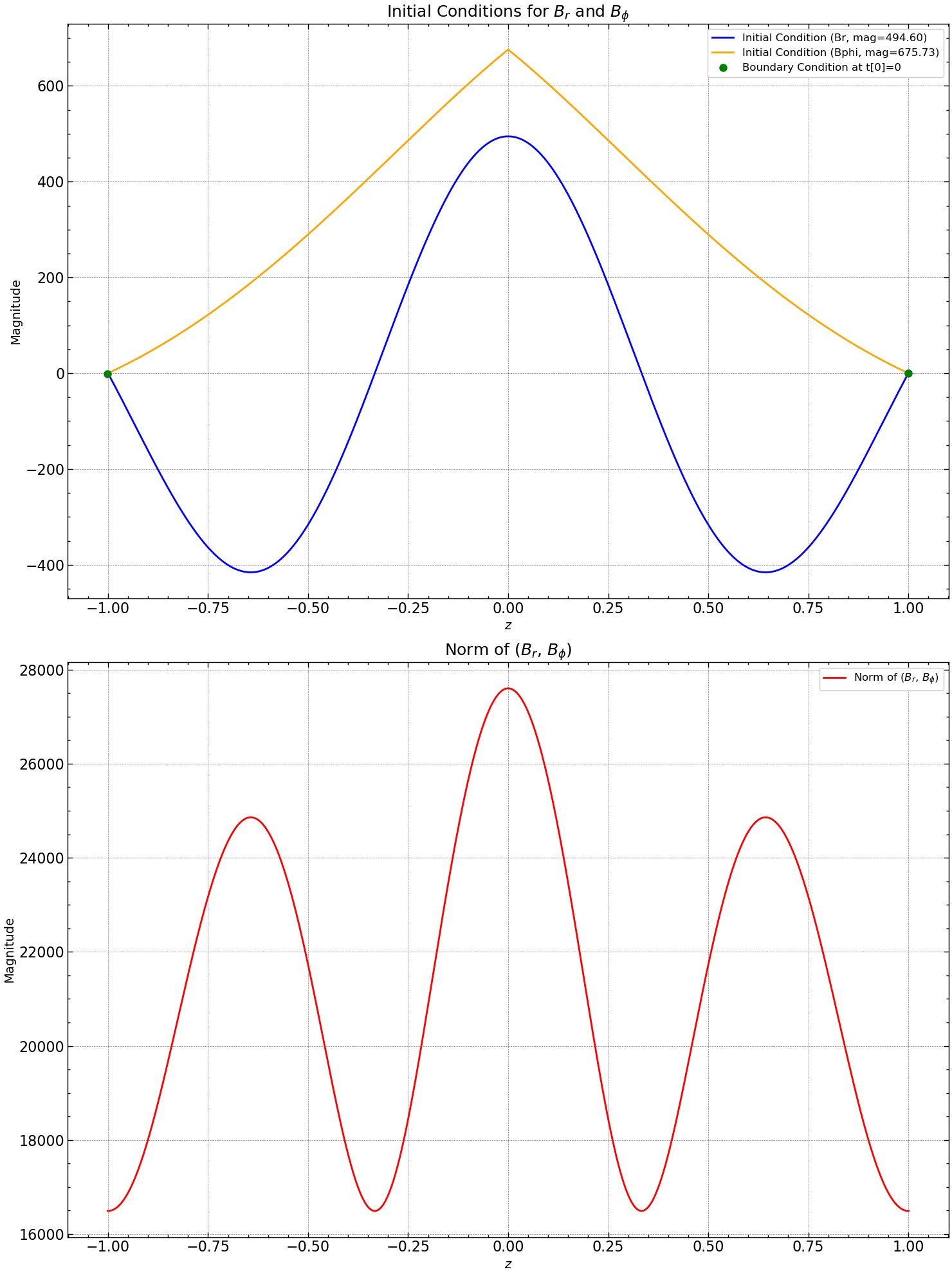
Discrete Initial and Boundary Conditions#

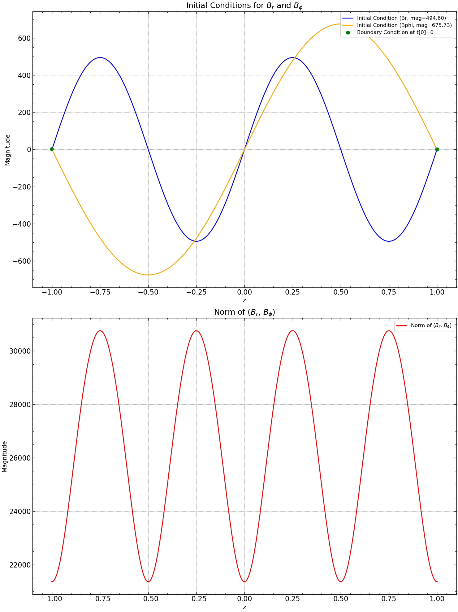
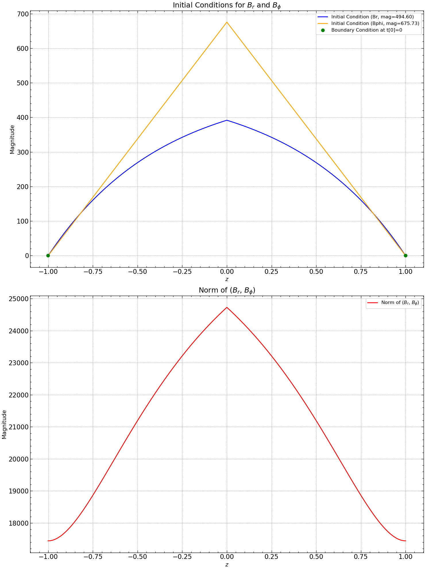
The discrete initial conditions are $B[i,0]= B_o sin(\gamma z[i])$ and the discrete boundary conditions are

\[\frac{\partial B[0,j]}{\partial z} = \frac{\partial B[N,j]}{\partial z} = 0\]

where $B[i,j]$ is the numerical approximation of $B(x[i],t[j])$. We have now used the exact eigensolution for the initial condition, denoted by B at $t=0$. While we have experimented with other initial conditions, this specific choice corresponds to the physical solution and will therefore provide the best results. The Figure below plots values of $B[i,0]$ for the initial (blue) and boundary (red) conditions for $t[0]=0$.

def generate_random_Bo(seed_value):
    np.random.seed(seed_value)  
    random_float = np.random.rand()  
    return random_float

def initial_conditions(N, time_steps, seed_value, m, n, BCtype="neumann"):
    mag_br = 1000*generate_random_Bo(seed_value)
    mag_bphi = 1000*generate_random_Bo(seed_value + 1)  

    # Extend z to include ghost zones
    z = np.linspace(-1 - 2/N, 1 + 2/N, N+2)
    h = z[1] - z[0]

    Br = np.zeros((N+2, time_steps+1))
    Bphi = np.zeros((N+2, time_steps+1))
    b1 = np.zeros(N)
    b2 = np.zeros(N)

    # Initial Condition for Br and Bphi
    for i in range(1, N+1):
        Br[i, 0] = mag_br * np.sin((m) * np.pi * z[i])
        Bphi[i, 0] = mag_bphi * np.sin((n) * np.pi * z[i])
    # Apply Neumann boundary conditions
    if BCtype == "neumann":
        Br[0, :] = Br[2, :]
        Br[N+1, :] = Br[N -1, :]
        Bphi[0, :] = Bphi[2, :]
        Bphi[N+1, :] = Bphi[N -1, :]

    return z, Br, Bphi, b1, b2, mag_br, mag_bphi

# Update the initial conditions
seed_value = 50
m, n = 2, 1
z, Br, Bphi, b1, b2, mag_br, mag_bphi = initial_conditions(N, time_steps, seed_value, m, n, BCtype="neumann")

fig, axs = plt.subplots(2, figsize=(15, 20))

axs[0].plot(z, Br[:, 0], label=f'Initial Condition (Br, mag={mag_br:.2f})', color='blue')
axs[0].plot(z, Bphi[:,0], label=f'Initial Condition (Bphi, mag={mag_bphi:.2f})', color='orange')
axs[0].plot(z[[0, N]], Br[[0, N], 0], 'go', markersize=8, label='Boundary Condition at t[0]=0')
axs[0].set_title(r'Initial Conditions for $B_{r}$ and $B_{\phi}$', fontsize=18)
axs[0].set_xlabel(r'$z$', fontsize=14)
axs[0].set_ylabel('Magnitude', fontsize=14)
axs[0].legend(loc='upper right', fontsize=12)
axs[0].grid(True, linestyle='--', alpha=0.5)


norm_Br_Bphi = [np.linalg.norm(np.sqrt(Br[i, 0]**2 + Bphi[:,0]**2)) for i in range(len(z))]
axs[1].plot(z, norm_Br_Bphi , label=r'Norm of ($B_r$, $B_{\phi}$)', linestyle='-', color='red')
axs[1].set_title(r'Norm of ($B_{r}$, $B_{\phi}$)', fontsize=18)
axs[1].set_xlabel(r'$z$', fontsize=14)
axs[1].set_ylabel('Magnitude', fontsize=14)
axs[1].legend(loc='upper right', fontsize=12)
axs[1].grid(True, linestyle='--', alpha=0.5)

plt.tight_layout()
plt.savefig("seed_1/initial_conditions_neu.pdf")
plt.show()

../../_images/8d64a34f3c57cff3040e5055ec3b617fe63635f2b022e08d438e1425df818e2a.png

Discretized Equations#

Using finite difference approximations, we discretize the time derivatives and the second-order spatial derivatives in the given PDEs.

Let $B_i$ represent $B_r$ and $B_\phi$ for $i = 1, 2, \ldots, N$.

The discretized equations for $B_i$ and $B_{N+i}$ are:

For $B_r$: $$ \frac{B_i^{j+1} - B_i^{j}}{k} = \eta_t \frac{1}{2} \left( \frac{B_{i-1}^{j+1} - 2B_{i}^{j+1} + B_{i+1}^{j+1} + B_{i-1}^{j} - 2B_{i}^{j} + B_{i+1}^{j}}{h^2} \right) $$
For $B_\phi$: $$ \frac{B_{N+i}^{j+1} - B_{N+i}^{j}}{k} = \eta_t \frac{1}{2} \left( \frac{B_{N+i-1}^{j+1} - 2B_{N+i}^{j+1} + B_{N+i+1}^{j+1} + B_{N+i-1}^{j} - 2B_{N+i}^{j} + B_{N+i+1}^{j}}{h^2} \right) $$

We could redefine a few parameters for the ease of this matrix representation. They are the following:

\[ \alpha = \frac{\eta_t k}{2 h^2} \]

After rearranging $j + 1$ terms on one side and $j$ terms on the other side of the equation, we get the following sets of linear equations:

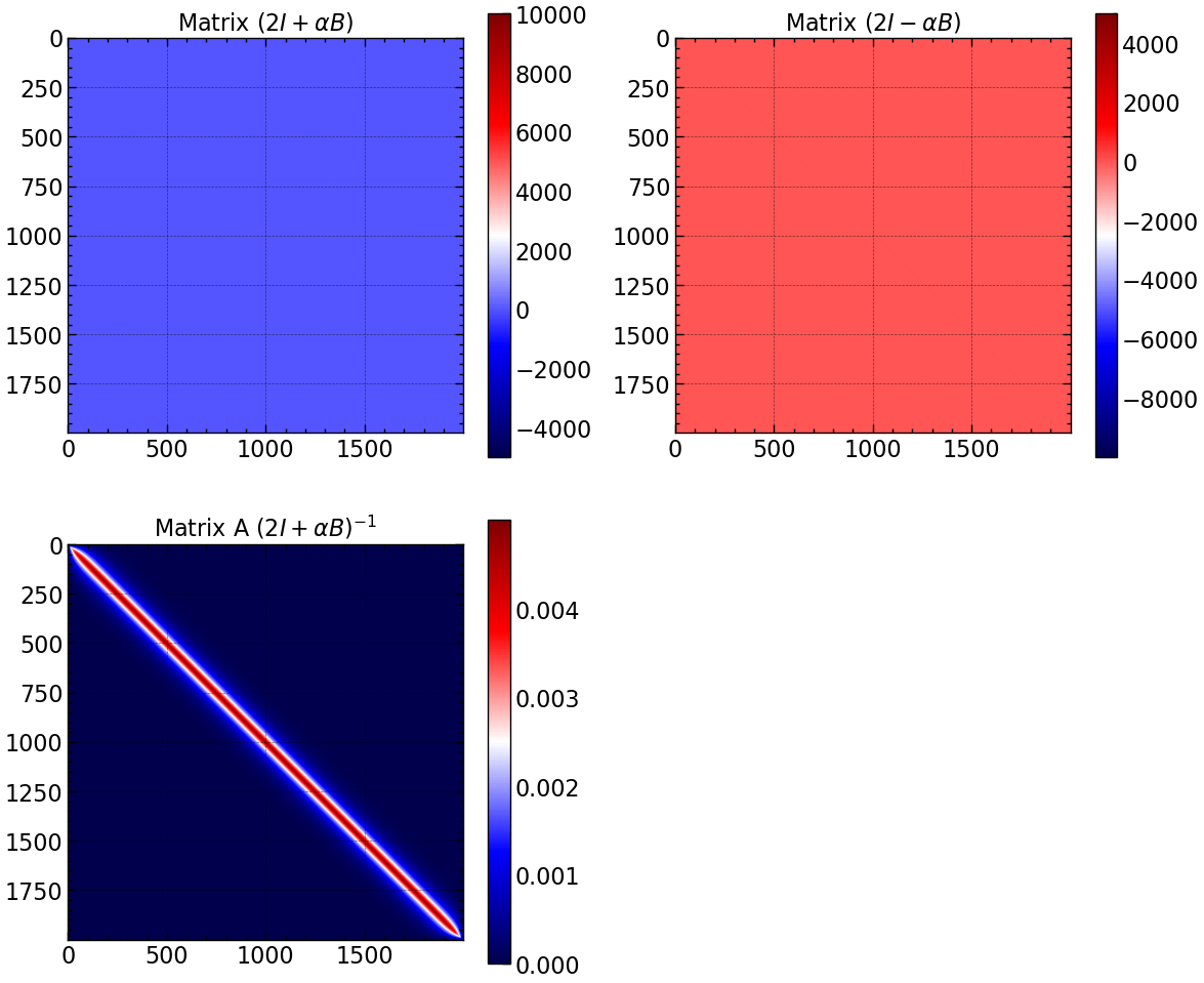
\[ -\alpha B_{i-1j+1} + ( 2 + 2\alpha)B_{ij+1} - \alpha B_{i+1j+1} = \alpha B_{i-1j} + (2-2\alpha)B_{ij} + \alpha B_{i+1j} \]

\[ (2I + \alpha A)\mathbf{B}_{j} = (2I - \alpha A)\mathbf{B}_{j-1} +\mathbf{b}_{j}+\mathbf{b}_{j-1} \]

for which $T$ is a $N-2 \times N-2$ matrix:

\[\begin{split} (2I + \alpha A) = \begin{pmatrix} 2+2\alpha & -\alpha & 0 & 0 & 0 & 0 & 0 & 0 \\ -\alpha & 2+2\alpha & -\alpha & 0 & 0 & 0 & 0 & 0 \\ 0 & -\alpha & 2+2\alpha & -\alpha & 0 & 0 & 0 & 0 \\ 0 & 0 & -\alpha & 2+2\alpha & -\alpha & 0 & 0 & 0 \\ 0 & 0 & 0 & -\alpha & 2+2\alpha & -\alpha & 0 & 0 \\ 0 & 0 & 0 & 0 & -\alpha & 2+2\alpha & -\alpha & 0 \\ 0 & 0 & 0 & 0 & 0 & -\alpha & 2+2\alpha & -\alpha \\ 0 & 0 & 0 & 0 & 0 & 0 & -\alpha & 2+2\alpha \\ \end{pmatrix} \end{split}\]

$S$ is another $N-2 \times N-2$ matrix:

\[\begin{split} (2I - \alpha A) = \begin{pmatrix} 2-2\alpha & \alpha & 0 & 0 & 0 & 0 & 0 & 0 \\ \alpha & 2-2\alpha & \alpha & 0 & 0 & 0 & 0 & 0 \\ 0 & \alpha & 2-2\alpha & \alpha & 0 & 0 & 0 & 0 \\ 0 & 0 & \alpha & 2-2\alpha & \alpha & 0 & 0 & 0 \\ 0 & 0 & 0 & \alpha & 2-2\alpha & \alpha & 0 & 0 \\ 0 & 0 & 0 & 0 & \alpha & 2-2\alpha & \alpha & 0 \\ 0 & 0 & 0 & 0 & 0 & \alpha & 2-2\alpha & \alpha \\ 0 & 0 & 0 & 0 & 0 & 0 & \alpha & 2-2\alpha \\ \end{pmatrix} \end{split}\]

$\mathbf{B}_j$ is a column vector of size N-2 containing $B_{ij}$ values, $\mathbf{b}_j$ and $\mathbf{b}_{j-1}$ are column vectors of size N-2 representing the boundary conditions for the current and next time steps, respectively.

#  A and B
A = np.zeros((N, N))
B = np.zeros((N, N))
for i in range(N):
    if i == 0 or i == N-1:
        A[i, i] = 1 + r
        B[i, i] = 1 - r
    A[i, i] = 2 + 2 * r
    B[i, i] = 2 - 2 * r
    if i < N-1:
        A[i, i+1] = -r
        A[i+1, i] = -r
        B[i, i+1] = r
        B[i+1, i] = r

# inverse of A
A_inv = np.linalg.inv(A)

fig, axs = plt.subplots(2, 2, figsize=(12, 10))
im = axs[0, 0].imshow(A, cmap='seismic')
axs[0, 0].set_title(r'Matrix $(2I + \alpha B)$')
plt.colorbar(im, ax=axs[0, 0])
im = axs[0, 1].imshow(B, cmap='seismic')
axs[0, 1].set_title(r'Matrix $(2I - \alpha B)$')
plt.colorbar(im, ax=axs[0, 1])
im = axs[1, 0].imshow(A_inv, cmap='seismic')
axs[1, 0].set_title(r'Matrix A $(2I + \alpha B)^{-1}$')
plt.colorbar(im, ax=axs[1, 0])
axs[1, 1].axis('off')

plt.tight_layout()
plt.savefig("seed_1/matrix_A_B_A_inv_neu.pdf")
plt.show()

../../_images/dac0c004478a36b6fd40093f980b11fffc33681ea73d1f6a08d1f24d57556e15.png

for j in range (1,time_steps+1):
    b1[0]=r*Br[0,j-1]+r*Br[0,j]
    b1[N-2]=r*Br[N+1,j-1]+r*Br[N+1,j]
    v1=np.dot(B,Br[1:(N+1),j-1])
    Br[1:(N+1),j]=np.dot(A_inv,v1+b1)
    
    b2[0]=r*Bphi[0,j-1]+r*Bphi[0,j]
    b2[N-1]=r*Bphi[N+1,j-1]+r*Bphi[N+1,j]
    v2=np.dot(B,Bphi[1:(N+1),j-1])
    Bphi[1:(N+1),j]=np.dot(A_inv,v2+b2)

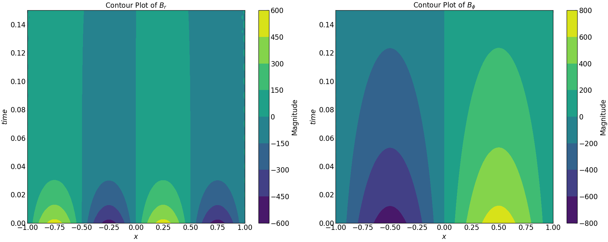
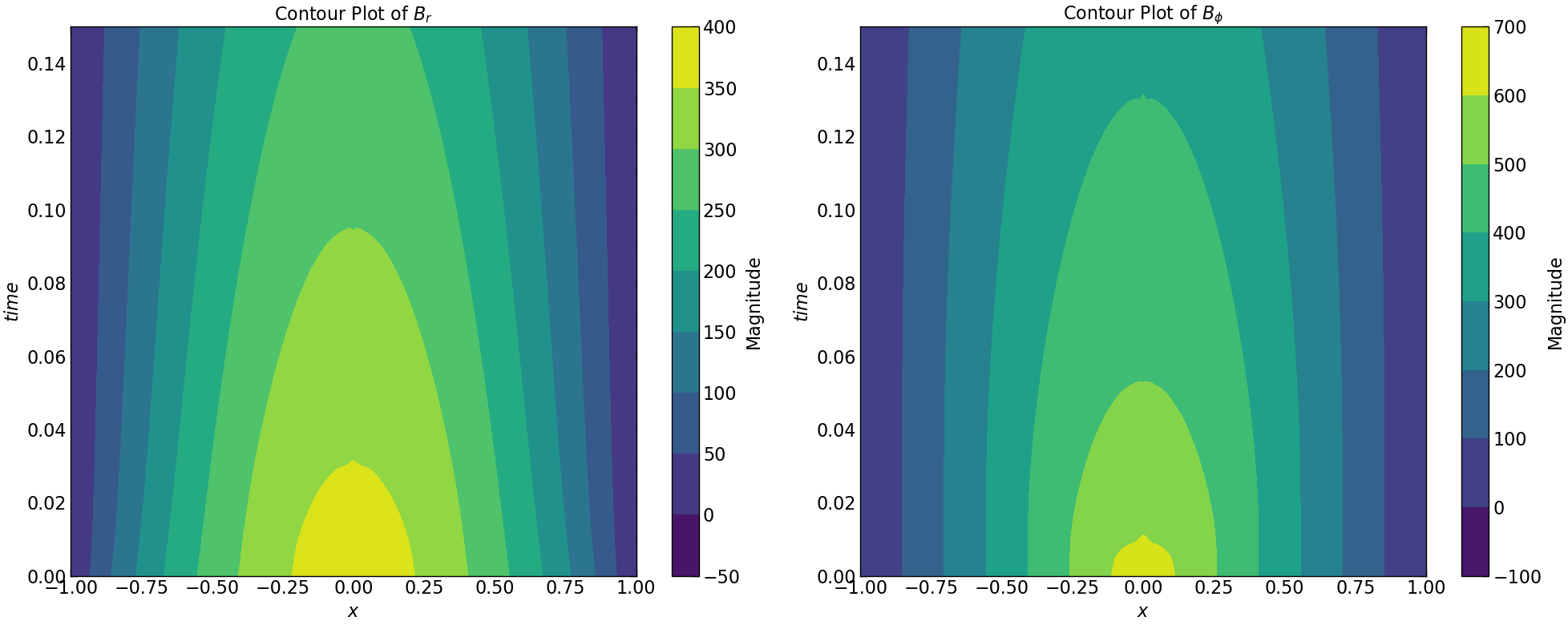
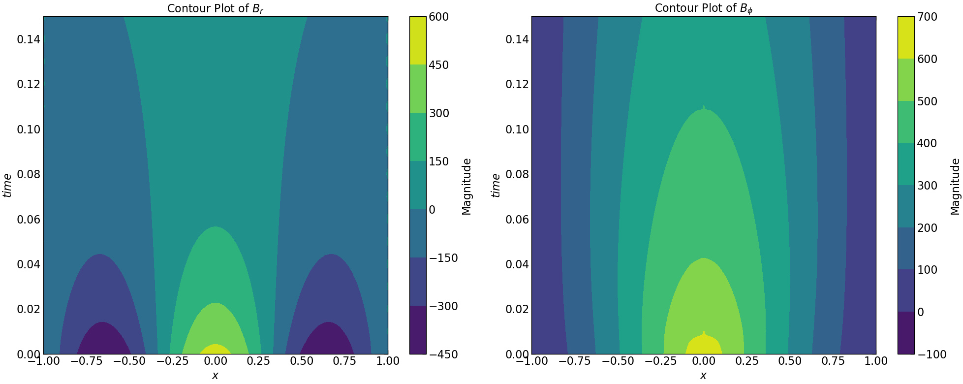
# Plotting Br
plt.figure(figsize=(20, 8))

plt.subplot(1, 2, 1)
plt.contourf(Z1, Y1, Br.transpose(), cmap='viridis')
plt.colorbar(label='Magnitude')
plt.xlabel(r'$x$')
plt.ylabel(r'$time$')
plt.title(r'Contour Plot of $B_r$')

# Plotting Bphi
plt.subplot(1, 2, 2)
plt.contourf(Z1, Y1, Bphi.transpose(), cmap='viridis')
plt.colorbar(label='Magnitude')
plt.xlabel(r'$x$')
plt.ylabel(r'$time$')
plt.title(r'Contour Plot of $B_{\phi}$')

plt.tight_layout()
plt.savefig("seed_1/contour_plot_Br_Bphi_neu.pdf")
plt.show()

../../_images/2cd8a9f8ecda383d1794247b56daa7abd3a31d464e75c01ea4cd13d14d9983d1.png

norm_squared_sum = np.sqrt(Br**2 + Bphi**2)
pitch_angle = np.arctan2(Br, Bphi) * (180 / np.pi)

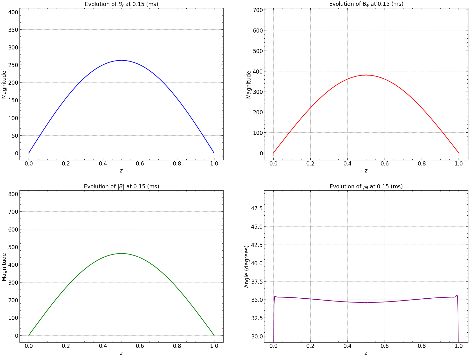
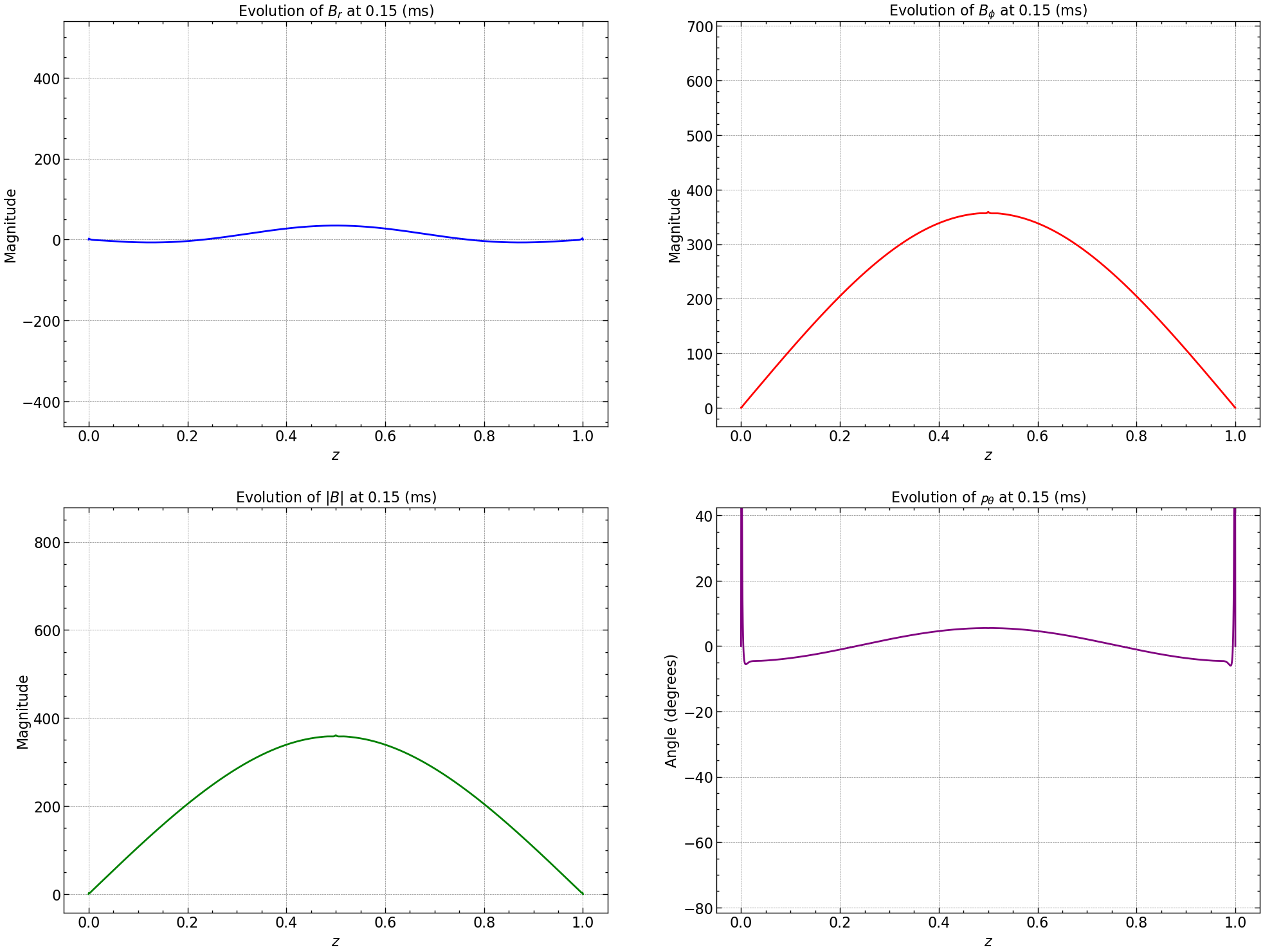
fig, axs = plt.subplots(2, 2, figsize=(24, 18))
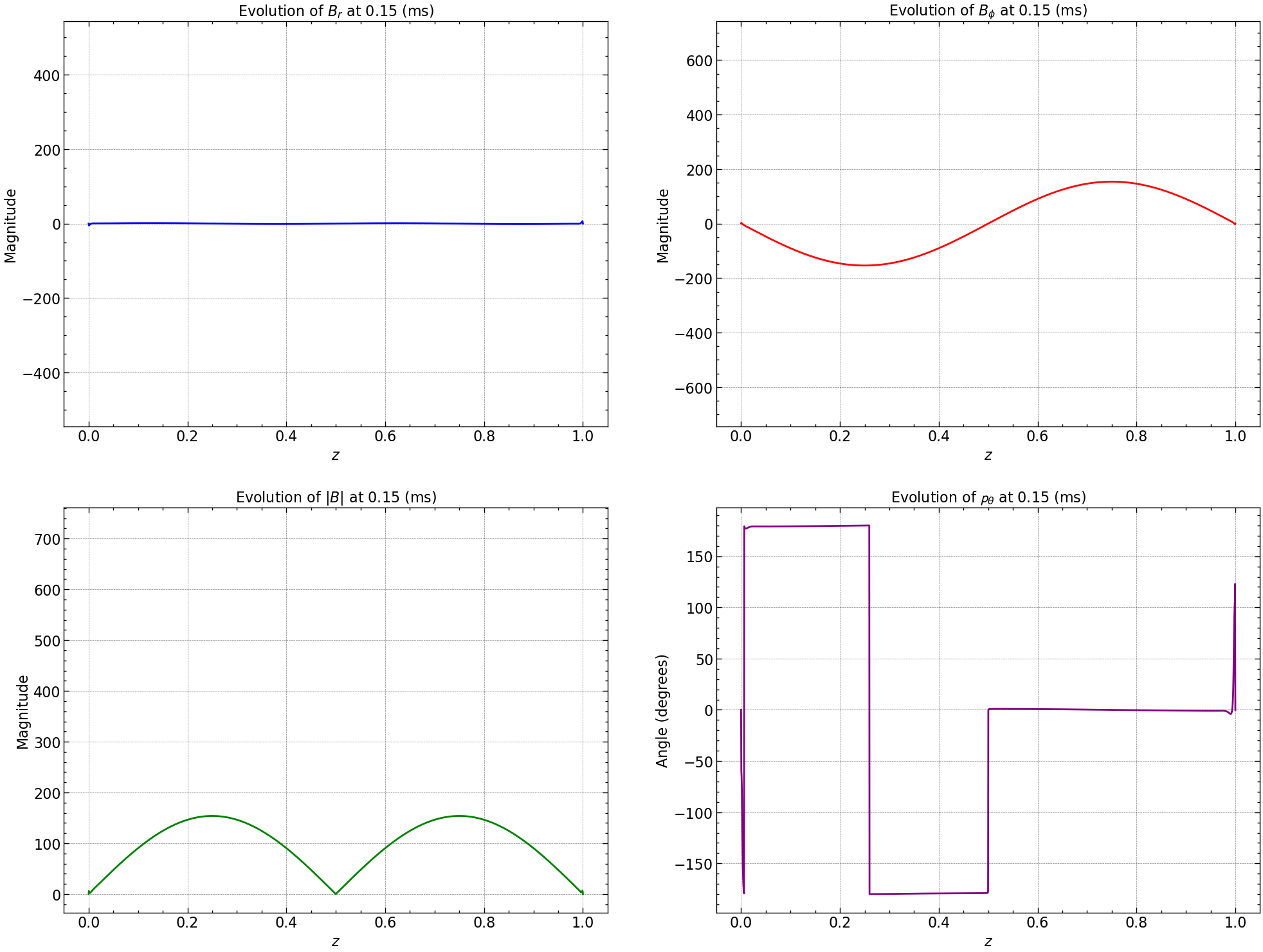
# Plot Br
line_br, = axs[0, 0].plot(np.linspace(0, 1, Br.shape[0]), Br[:, 0], color='blue', label='Br')
axs[0, 0].set_xlabel(r'$z$')
axs[0, 0].set_ylabel('Magnitude')
axs[0, 0].set_title(r'Evolution of $B_r$')

# Plot Bphi
line_bphi, = axs[0, 1].plot(np.linspace(0, 1, Bphi.shape[0]), Bphi[:, 0], color='red', label='Bphi')
axs[0, 1].set_xlabel(r'$z$')
axs[0, 1].set_ylabel('Magnitude')
axs[0, 1].set_title(r'Evolution of $B_{\phi}$')

# Plot Norm
line_norm, = axs[1, 0].plot(np.linspace(0, 1, norm_squared_sum.shape[0]), norm_squared_sum[:, 0], color='green', label='Norm')
axs[1, 0].set_xlabel(r'$z$')
axs[1, 0].set_ylabel('Magnitude')
axs[1, 0].set_title(r'Evolution of $|B|$')


line_pitch, = axs[1, 1].plot(np.linspace(0, 1, pitch_angle.shape[0]), pitch_angle[:, 0], color='purple', label='Pitch Angle')
axs[1, 1].set_xlabel(r'$z$')
axs[1, 1].set_ylabel('Angle (degrees)')
axs[1, 1].set_title(r'Evolution of Pitch Angle ($\mathbf{p}_{\theta}$)')

def update(frame):
    time = frame * k
    line_br.set_ydata(Br[:, frame])
    axs[0, 0].set_title(r'Evolution of $B_r$ at %s (ms)' % time)
    
    line_bphi.set_ydata(Bphi[:, frame])
    axs[0, 1].set_title(r'Evolution of $B_{\phi}$ at %s (ms)' % time)
    
    line_norm.set_ydata(norm_squared_sum[:, frame])
    axs[1, 0].set_title(r'Evolution of $|B|$ at %s (ms)' % time)
    
    line_pitch.set_ydata(pitch_angle[:, frame])
    axs[1, 1].set_title(r'Evolution of $\mathcal{p}_{\theta}$ at %s (ms)' % time)
    
    return line_br, line_bphi, line_norm, line_pitch

ani = FuncAnimation(fig, update, frames=range(Br.shape[1]), interval=70)
ani.save('seed_1/Br_Bphi_Norm_Pitch_evolution_neu.gif', writer='pillow')

plt.show()

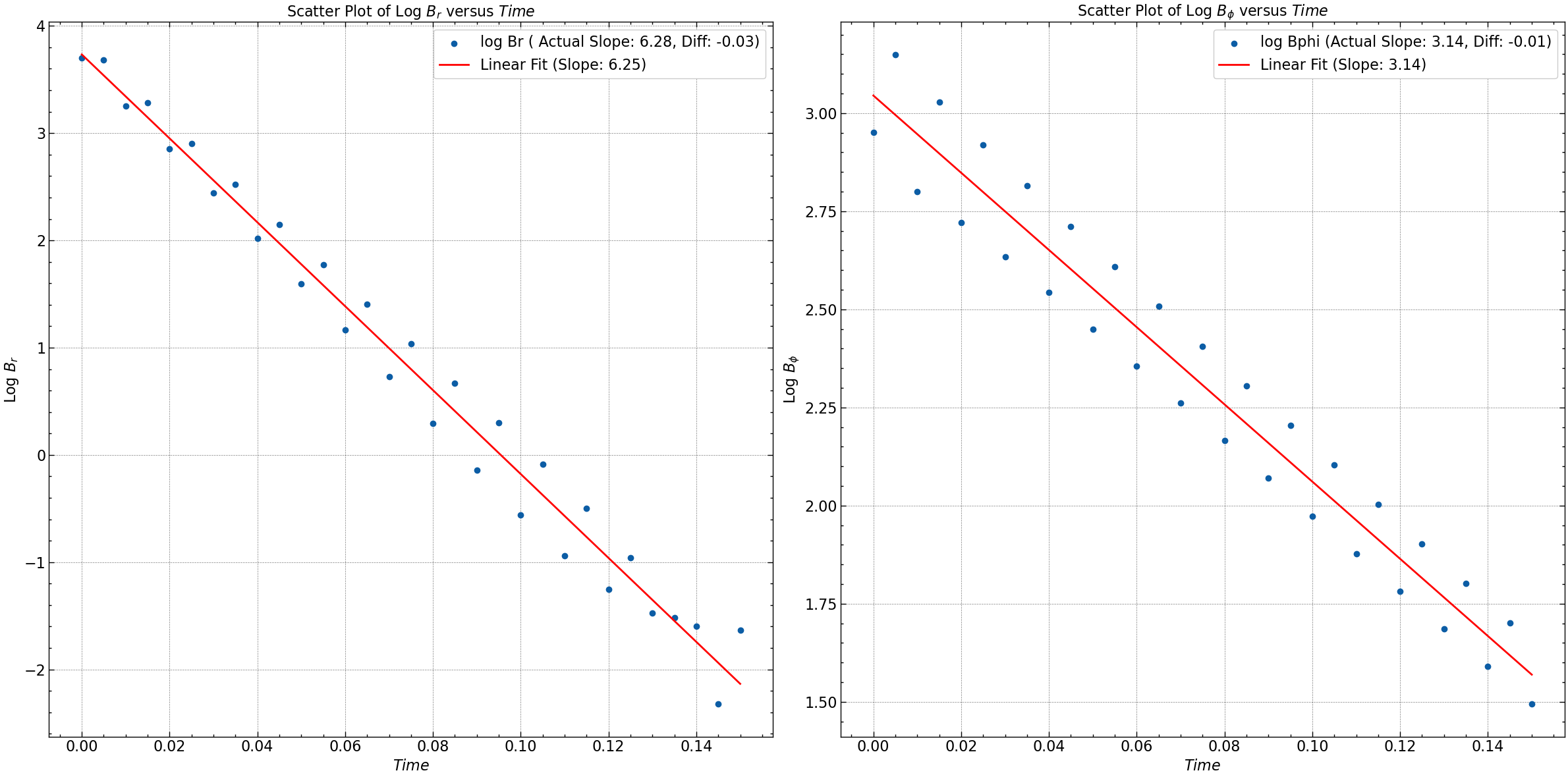
../../_images/8ca5dfc4cbfbe1d79a07c816eb01c0f2dbbd0a01c8a97ffd68f2ab8070a015cd.png

log_Br = np.log(np.abs(Br[14]))
log_Bphi = np.log(np.abs(Bphi[10]))

slope_Br, intercept_Br = np.polyfit(time, log_Br, 1)
slope_Bphi, intercept_Bphi = np.polyfit(time, log_Bphi, 1)

actual_slope_Br = (m)* np.pi  
actual_slope_Bphi = (n)* np.pi

difference_Br = np.sqrt(-slope_Br) - actual_slope_Br
difference_Bphi = np.sqrt(-slope_Bphi) - actual_slope_Bphi

print(f"Br: Actual Slope = {actual_slope_Br}, Computed Slope = {np.sqrt(-slope_Br)}, Difference = {difference_Br}")
print(f"Bphi: Actual Slope = {actual_slope_Bphi}, Computed Slope = {np.sqrt(-slope_Bphi)}, Difference = {difference_Bphi}")

Br: Actual Slope = 6.283185307179586, Computed Slope = 6.254304244389971, Difference = -0.02888106278961544
Bphi: Actual Slope = 3.141592653589793, Computed Slope = 3.1364343755193484, Difference = -0.005158278070444666

plt.figure(figsize=(24, 12))

# Scatter plot for log Br
plt.subplot(1, 2, 1)
plt.scatter(time, log_Br, label=f'log Br ( Actual Slope: {actual_slope_Br:.2f}, Diff: {difference_Br:.2f})')
plt.xlabel(r'$Time$')
plt.ylabel(r'Log $B_r$')
plt.title(r'Scatter Plot of Log $B_r$ versus $Time$')
plt.grid(True)

# Linear fit for log Br
fit_Br = np.polyfit(time, log_Br, 1)
plt.plot(time, np.polyval(fit_Br, time), color='red', label=f'Linear Fit (Slope: {np.sqrt(-fit_Br[0]):.2f})')
plt.legend()

# Scatter plot for log Bphi
plt.subplot(1, 2, 2)
plt.scatter(time, log_Bphi, label=f'log Bphi (Actual Slope: {actual_slope_Bphi:.2f}, Diff: {difference_Bphi:.2f})')
plt.xlabel(r'$Time$')
plt.ylabel(r'Log $B_{\phi}$')
plt.title(r'Scatter Plot of Log $B_{\phi}$ versus $Time$')
plt.grid(True)

# Linear fit for log Bphi
fit_Bphi = np.polyfit(time, log_Bphi, 1)
plt.plot(time, np.polyval(fit_Bphi, time), color='red', label=f'Linear Fit (Slope: {np.sqrt(-fit_Bphi[0]):.2f})')
plt.legend()

plt.tight_layout()
plt.savefig("seed_1/log_Br_Bphi_vs_time_neu.png")
plt.show()

../../_images/2a6b907b8cab31d324d87033a2c71480155c4511df8d75a31c72509db07dfbb3.png

Seed 2: Exponential Decay Solution

\[ B_r = B_o (1- e^{-\gamma(1-|z|)}) \]

\[ B_{\phi} = B_o (1 - \gamma|z|) \]

def generate_random_Bo(seed_value):
    np.random.seed(seed_value)  
    random_float = np.random.rand()  
    return random_float

def initial_conditions(N, time_steps, seed_value, gamma, BCtype="neumann"):
    mag_br = 1000*generate_random_Bo(seed_value)
    mag_bphi = 1000*generate_random_Bo(seed_value + 1)  

    # Extend z to include ghost zones
    z = np.linspace(-1 - 2/N, 1 + 2/N, N+2)
    h = z[1] - z[0]

    Br = np.zeros((N+2, time_steps+1))
    Bphi = np.zeros((N+2, time_steps+1))
    b1 = np.zeros(N)
    b2 = np.zeros(N)

    # Initial Condition for Br and Bphi
    for i in range(1, N+1):
        Br[i, 0] = mag_br * (1 - np.exp( -gamma * (1-np.abs(z[i]))))
        Bphi[i, 0] = mag_bphi * (1 - np.abs(z[i]))
    # Apply Neumann boundary conditions
    if BCtype == "neumann":
        Br[0, :] = Br[2, :]
        Br[N+1, :] = Br[N -1, :]
        Bphi[0, :] = Bphi[2, :]
        Bphi[N+1, :] = Bphi[N -1, :]

    return z, Br, Bphi, b1, b2, mag_br, mag_bphi

# Update the initial conditions
seed_value = 50
gamma = np.pi/2
z, Br, Bphi, b1, b2, mag_br, mag_bphi = initial_conditions(N, time_steps, seed_value, gamma, BCtype="neumann")

fig, axs = plt.subplots(2, figsize=(15, 20))

axs[0].plot(z, Br[:, 0], label=f'Initial Condition (Br, mag={mag_br:.2f})', color='blue')
axs[0].plot(z, Bphi[:,0], label=f'Initial Condition (Bphi, mag={mag_bphi:.2f})', color='orange')
axs[0].plot(z[[0, N]], Br[[0, N], 0], 'go', markersize=8, label='Boundary Condition at t[0]=0')
axs[0].set_title(r'Initial Conditions for $B_{r}$ and $B_{\phi}$', fontsize=18)
axs[0].set_xlabel(r'$z$', fontsize=14)
axs[0].set_ylabel('Magnitude', fontsize=14)
axs[0].legend(loc='upper right', fontsize=12)
axs[0].grid(True, linestyle='--', alpha=0.5)


norm_Br_Bphi = [np.linalg.norm(np.sqrt(Br[i, 0]**2 + Bphi[:,0]**2)) for i in range(len(z))]
axs[1].plot(z, norm_Br_Bphi , label=r'Norm of ($B_r$, $B_{\phi}$)', linestyle='-', color='red')
axs[1].set_title(r'Norm of ($B_{r}$, $B_{\phi}$)', fontsize=18)
axs[1].set_xlabel(r'$z$', fontsize=14)
axs[1].set_ylabel('Magnitude', fontsize=14)
axs[1].legend(loc='upper right', fontsize=12)
axs[1].grid(True, linestyle='--', alpha=0.5)

plt.tight_layout()
plt.savefig("seed_2/initial_conditions_neu.pdf")
plt.show()

../../_images/a919c53d93ebaade0c904e8feba2776635c300553d588f7a9a90d3707d22195c.png

#  A and B
A = np.zeros((N, N))
B = np.zeros((N, N))
for i in range(N):
    if i == 0 or i == N-1:
        A[i, i] = 1 + r
        B[i, i] = 1 - r
    A[i, i] = 2 + 2 * r
    B[i, i] = 2 - 2 * r
    if i < N-1:
        A[i, i+1] = -r
        A[i+1, i] = -r
        B[i, i+1] = r
        B[i+1, i] = r

# inverse of A
A_inv = np.linalg.inv(A)

fig, axs = plt.subplots(2, 2, figsize=(12, 10))
im = axs[0, 0].imshow(A, cmap='seismic')
axs[0, 0].set_title(r'Matrix $(2I + \alpha B)$')
plt.colorbar(im, ax=axs[0, 0])
im = axs[0, 1].imshow(B, cmap='seismic')
axs[0, 1].set_title(r'Matrix $(2I - \alpha B)$')
plt.colorbar(im, ax=axs[0, 1])
im = axs[1, 0].imshow(A_inv, cmap='seismic')
axs[1, 0].set_title(r'Matrix A $(2I + \alpha B)^{-1}$')
plt.colorbar(im, ax=axs[1, 0])
axs[1, 1].axis('off')

plt.tight_layout()
plt.savefig("seed_2/matrix_A_B_A_inv_neu.pdf")
plt.show()

for j in range (1,time_steps+1):
    b1[0]=r*Br[0,j-1]+r*Br[0,j]
    b1[N-2]=r*Br[N+1,j-1]+r*Br[N+1,j]
    v1=np.dot(B,Br[1:(N+1),j-1])
    Br[1:(N+1),j]=np.dot(A_inv,v1+b1)
    
    b2[0]=r*Bphi[0,j-1]+r*Bphi[0,j]
    b2[N-1]=r*Bphi[N+1,j-1]+r*Bphi[N+1,j]
    v2=np.dot(B,Bphi[1:(N+1),j-1])
    Bphi[1:(N+1),j]=np.dot(A_inv,v2+b2)

# Plotting Br
plt.figure(figsize=(20, 8))

plt.subplot(1, 2, 1)
plt.contourf(Z1, Y1, Br.transpose(), cmap='viridis')
plt.colorbar(label='Magnitude')
plt.xlabel(r'$x$')
plt.ylabel(r'$time$')
plt.title(r'Contour Plot of $B_r$')

# Plotting Bphi
plt.subplot(1, 2, 2)
plt.contourf(Z1, Y1, Bphi.transpose(), cmap='viridis')
plt.colorbar(label='Magnitude')
plt.xlabel(r'$x$')
plt.ylabel(r'$time$')
plt.title(r'Contour Plot of $B_{\phi}$')

plt.tight_layout()
plt.savefig("seed_2/contour_plot_Br_Bphi_neu.pdf")
plt.show()

../../_images/a45a35f3c3ee772cc8c9d8091321819621cf5793c42df241a8166c1dfc1654ba.png

norm_squared_sum = np.sqrt(Br**2 + Bphi**2)
pitch_angle = np.arctan2(Br, Bphi) * (180 / np.pi)

fig, axs = plt.subplots(2, 2, figsize=(24, 18))
# Plot Br
line_br, = axs[0, 0].plot(np.linspace(0, 1, Br.shape[0]), Br[:, 0], color='blue', label='Br')
axs[0, 0].set_xlabel(r'$z$')
axs[0, 0].set_ylabel('Magnitude')
axs[0, 0].set_title(r'Evolution of $B_r$')

# Plot Bphi
line_bphi, = axs[0, 1].plot(np.linspace(0, 1, Bphi.shape[0]), Bphi[:, 0], color='red', label='Bphi')
axs[0, 1].set_xlabel(r'$z$')
axs[0, 1].set_ylabel('Magnitude')
axs[0, 1].set_title(r'Evolution of $B_{\phi}$')

# Plot Norm
line_norm, = axs[1, 0].plot(np.linspace(0, 1, norm_squared_sum.shape[0]), norm_squared_sum[:, 0], color='green', label='Norm')
axs[1, 0].set_xlabel(r'$z$')
axs[1, 0].set_ylabel('Magnitude')
axs[1, 0].set_title(r'Evolution of $|B|$')


line_pitch, = axs[1, 1].plot(np.linspace(0, 1, pitch_angle.shape[0]), pitch_angle[:, 0], color='purple', label='Pitch Angle')
axs[1, 1].set_xlabel(r'$z$')
axs[1, 1].set_ylabel('Angle (degrees)')
axs[1, 1].set_title(r'Evolution of Pitch Angle ($\mathbf{p}_{\theta}$)')

def update(frame):
    time = frame * k
    line_br.set_ydata(Br[:, frame])
    axs[0, 0].set_title(r'Evolution of $B_r$ at %s (ms)' % time)
    
    line_bphi.set_ydata(Bphi[:, frame])
    axs[0, 1].set_title(r'Evolution of $B_{\phi}$ at %s (ms)' % time)
    
    line_norm.set_ydata(norm_squared_sum[:, frame])
    axs[1, 0].set_title(r'Evolution of $|B|$ at %s (ms)' % time)
    
    line_pitch.set_ydata(pitch_angle[:, frame])
    axs[1, 1].set_title(r'Evolution of $\mathcal{p}_{\theta}$ at %s (ms)' % time)
    
    return line_br, line_bphi, line_norm, line_pitch

ani = FuncAnimation(fig, update, frames=range(Br.shape[1]), interval=70)
ani.save('seed_2/Br_Bphi_Norm_Pitch_evolution_neu.gif', writer='pillow')

plt.show()

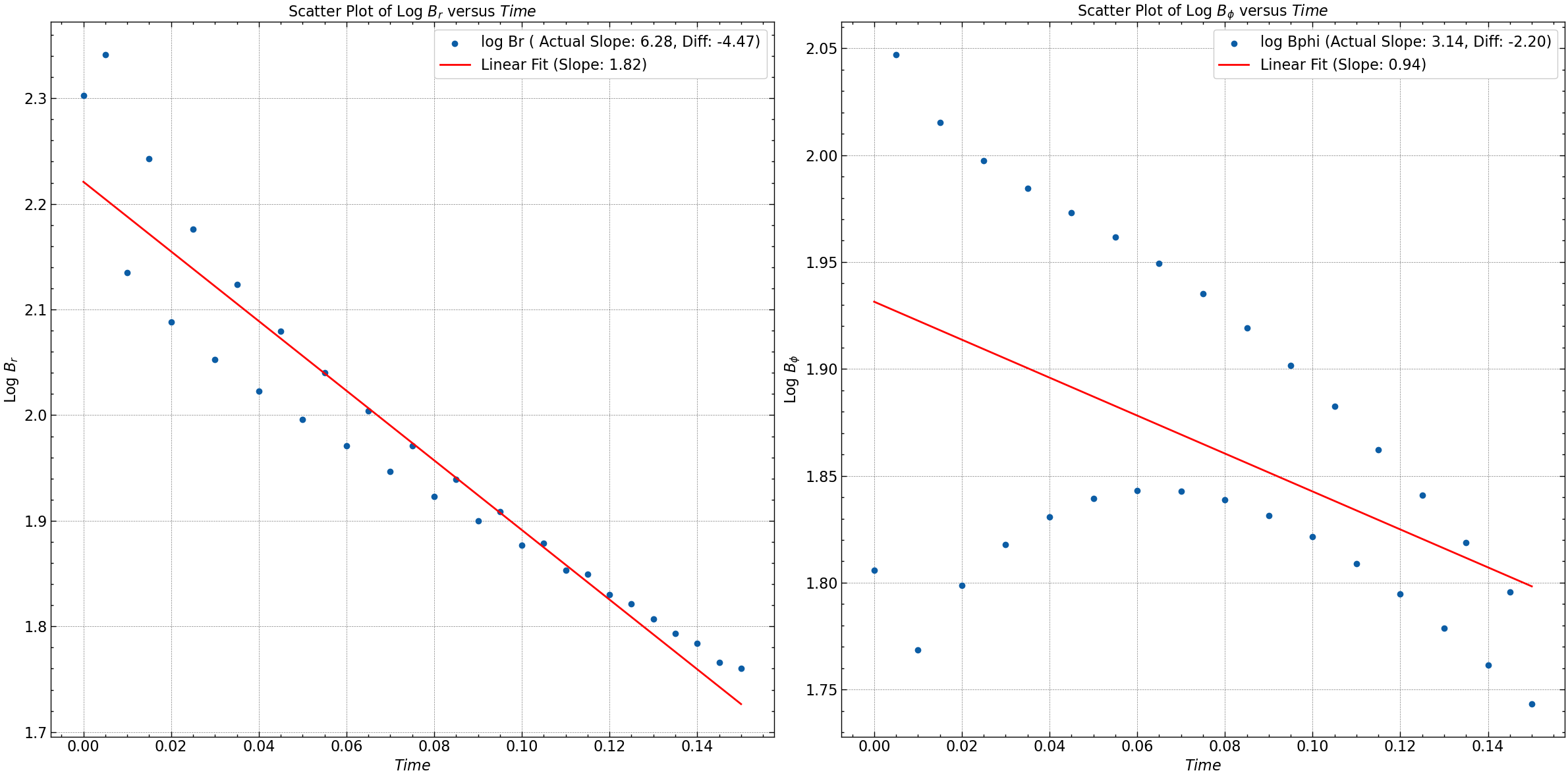
../../_images/9cc502ff736e9fa6cdd5f00cf0f0e14a80dac307b52313415872567106cf7e4d.png

log_Br = np.log(np.abs(Br[14]))
log_Bphi = np.log(np.abs(Bphi[10]))

slope_Br, intercept_Br = np.polyfit(time, log_Br, 1)
slope_Bphi, intercept_Bphi = np.polyfit(time, log_Bphi, 1)

actual_slope_Br = (m)* np.pi  
actual_slope_Bphi = (n)* np.pi

difference_Br = np.sqrt(-slope_Br) - actual_slope_Br
difference_Bphi = np.sqrt(-slope_Bphi) - actual_slope_Bphi

print(f"Br: Actual Slope = {actual_slope_Br}, Computed Slope = {np.sqrt(-slope_Br)}, Difference = {difference_Br}")
print(f"Bphi: Actual Slope = {actual_slope_Bphi}, Computed Slope = {np.sqrt(-slope_Bphi)}, Difference = {difference_Bphi}")

Br: Actual Slope = 6.283185307179586, Computed Slope = 1.8155264473203325, Difference = -4.467658859859254
Bphi: Actual Slope = 3.141592653589793, Computed Slope = 0.9420823986781074, Difference = -2.1995102549116856

plt.figure(figsize=(24, 12))

# Scatter plot for log Br
plt.subplot(1, 2, 1)
plt.scatter(time, log_Br, label=f'log Br ( Actual Slope: {actual_slope_Br:.2f}, Diff: {difference_Br:.2f})')
plt.xlabel(r'$Time$')
plt.ylabel(r'Log $B_r$')
plt.title(r'Scatter Plot of Log $B_r$ versus $Time$')
plt.grid(True)

# Linear fit for log Br
fit_Br = np.polyfit(time, log_Br, 1)
plt.plot(time, np.polyval(fit_Br, time), color='red', label=f'Linear Fit (Slope: {np.sqrt(-fit_Br[0]):.2f})')
plt.legend()

# Scatter plot for log Bphi
plt.subplot(1, 2, 2)
plt.scatter(time, log_Bphi, label=f'log Bphi (Actual Slope: {actual_slope_Bphi:.2f}, Diff: {difference_Bphi:.2f})')
plt.xlabel(r'$Time$')
plt.ylabel(r'Log $B_{\phi}$')
plt.title(r'Scatter Plot of Log $B_{\phi}$ versus $Time$')
plt.grid(True)

# Linear fit for log Bphi
fit_Bphi = np.polyfit(time, log_Bphi, 1)
plt.plot(time, np.polyval(fit_Bphi, time), color='red', label=f'Linear Fit (Slope: {np.sqrt(-fit_Bphi[0]):.2f})')
plt.legend()

plt.tight_layout()
plt.savefig("seed_2/log_Br_Bphi_vs_time_neu.png")
plt.show()

../../_images/92115334c21c852c83e09c1a621788b212933aff8dbfe1b97a157f129b42e058.png

Seed 3: Gaussian & Trigonometric Decay Solution

\[ B_r = B_o e^{-\left(\frac{z}{\sigma}\right)^2} \cdot \cos\left(\frac{3\pi z}{2}\right)\]

\[ B_{\phi} = B_o e^{-|z|} \cdot \cos\left(\frac{\pi z}{2}\right) \]

def generate_random_Bo(seed_value):
    np.random.seed(seed_value)  
    random_float = np.random.rand()  
    return random_float

def initial_conditions(N, time_steps, seed_value, sigma, BCtype="neumann"):
    mag_br = 1000*generate_random_Bo(seed_value)
    mag_bphi = 1000*generate_random_Bo(seed_value + 1)  

    # Extend z to include ghost zones
    z = np.linspace(-1 - 2/N, 1 + 2/N, N+2)
    h = z[1] - z[0]

    Br = np.zeros((N+2, time_steps+1))
    Bphi = np.zeros((N+2, time_steps+1))
    b1 = np.zeros(N)
    b2 = np.zeros(N)

    # Initial Condition for Br and Bphi
    for i in range(1, N+1):
        Br[i, 0] = mag_br * np.exp( - z[i]**2/sigma**2) * np.cos(3*np.pi/2 * z[i])
        Bphi[i, 0] = mag_bphi * np.exp(- np.abs(z[i])) * np.cos(np.pi/2 * z[i])
    # Apply Neumann boundary conditions
    if BCtype == "neumann":
        Br[0, :] = Br[2, :]
        Br[N+1, :] = Br[N -1, :]
        Bphi[0, :] = Bphi[2, :]
        Bphi[N+1, :] = Bphi[N -1, :]

    return z, Br, Bphi, b1, b2, mag_br, mag_bphi

# Update the initial conditions
seed_value = 50
sigma = np.pi/2
z, Br, Bphi, b1, b2, mag_br, mag_bphi = initial_conditions(N, time_steps, seed_value, gamma, BCtype="neumann")

fig, axs = plt.subplots(2, figsize=(15, 20))

axs[0].plot(z, Br[:, 0], label=f'Initial Condition (Br, mag={mag_br:.2f})', color='blue')
axs[0].plot(z, Bphi[:,0], label=f'Initial Condition (Bphi, mag={mag_bphi:.2f})', color='orange')
axs[0].plot(z[[0, N]], Br[[0, N], 0], 'go', markersize=8, label='Boundary Condition at t[0]=0')
axs[0].set_title(r'Initial Conditions for $B_{r}$ and $B_{\phi}$', fontsize=18)
axs[0].set_xlabel(r'$z$', fontsize=14)
axs[0].set_ylabel('Magnitude', fontsize=14)
axs[0].legend(loc='upper right', fontsize=12)
axs[0].grid(True, linestyle='--', alpha=0.5)


norm_Br_Bphi = [np.linalg.norm(np.sqrt(Br[i, 0]**2 + Bphi[:,0]**2)) for i in range(len(z))]
axs[1].plot(z, norm_Br_Bphi , label=r'Norm of ($B_r$, $B_{\phi}$)', linestyle='-', color='red')
axs[1].set_title(r'Norm of ($B_{r}$, $B_{\phi}$)', fontsize=18)
axs[1].set_xlabel(r'$z$', fontsize=14)
axs[1].set_ylabel('Magnitude', fontsize=14)
axs[1].legend(loc='upper right', fontsize=12)
axs[1].grid(True, linestyle='--', alpha=0.5)

plt.tight_layout()
plt.savefig("seed_3/initial_conditions_neu.pdf")
plt.show()

../../_images/5e789af938c15140101d6303ef20c3fc4264b77b1b3849a4c08baa2c30a2f337.png

#  A and B
A = np.zeros((N, N))
B = np.zeros((N, N))
for i in range(N):
    if i == 0 or i == N-1:
        A[i, i] = 1 + r
        B[i, i] = 1 - r
    A[i, i] = 2 + 2 * r
    B[i, i] = 2 - 2 * r
    if i < N-1:
        A[i, i+1] = -r
        A[i+1, i] = -r
        B[i, i+1] = r
        B[i+1, i] = r

# inverse of A
A_inv = np.linalg.inv(A)

fig, axs = plt.subplots(2, 2, figsize=(12, 10))
im = axs[0, 0].imshow(A, cmap='seismic')
axs[0, 0].set_title(r'Matrix $(2I + \alpha B)$')
plt.colorbar(im, ax=axs[0, 0])
im = axs[0, 1].imshow(B, cmap='seismic')
axs[0, 1].set_title(r'Matrix $(2I - \alpha B)$')
plt.colorbar(im, ax=axs[0, 1])
im = axs[1, 0].imshow(A_inv, cmap='seismic')
axs[1, 0].set_title(r'Matrix A $(2I + \alpha B)^{-1}$')
plt.colorbar(im, ax=axs[1, 0])
axs[1, 1].axis('off')

plt.tight_layout()
plt.savefig("seed_3/matrix_A_B_A_inv_neu.pdf")
plt.show()

for j in range (1,time_steps+1):
    b1[0]=r*Br[0,j-1]+r*Br[0,j]
    b1[N-2]=r*Br[N+1,j-1]+r*Br[N+1,j]
    v1=np.dot(B,Br[1:(N+1),j-1])
    Br[1:(N+1),j]=np.dot(A_inv,v1+b1)
    
    b2[0]=r*Bphi[0,j-1]+r*Bphi[0,j]
    b2[N-1]=r*Bphi[N+1,j-1]+r*Bphi[N+1,j]
    v2=np.dot(B,Bphi[1:(N+1),j-1])
    Bphi[1:(N+1),j]=np.dot(A_inv,v2+b2)

# Plotting Br
plt.figure(figsize=(20, 8))

plt.subplot(1, 2, 1)
plt.contourf(Z1, Y1, Br.transpose(), cmap='viridis')
plt.colorbar(label='Magnitude')
plt.xlabel(r'$x$')
plt.ylabel(r'$time$')
plt.title(r'Contour Plot of $B_r$')

# Plotting Bphi
plt.subplot(1, 2, 2)
plt.contourf(Z1, Y1, Bphi.transpose(), cmap='viridis')
plt.colorbar(label='Magnitude')
plt.xlabel(r'$x$')
plt.ylabel(r'$time$')
plt.title(r'Contour Plot of $B_{\phi}$')

plt.tight_layout()
plt.savefig("seed_2/contour_plot_Br_Bphi_neu.pdf")
plt.show()

../../_images/12a8678fae2a77ece9cf41c15266be66afe0c7aed51134cc0ebccfa0744a992c.png

norm_squared_sum = np.sqrt(Br**2 + Bphi**2)
pitch_angle = np.arctan2(Br, Bphi) * (180 / np.pi)

fig, axs = plt.subplots(2, 2, figsize=(24, 18))
# Plot Br
line_br, = axs[0, 0].plot(np.linspace(0, 1, Br.shape[0]), Br[:, 0], color='blue', label='Br')
axs[0, 0].set_xlabel(r'$z$')
axs[0, 0].set_ylabel('Magnitude')
axs[0, 0].set_title(r'Evolution of $B_r$')

# Plot Bphi
line_bphi, = axs[0, 1].plot(np.linspace(0, 1, Bphi.shape[0]), Bphi[:, 0], color='red', label='Bphi')
axs[0, 1].set_xlabel(r'$z$')
axs[0, 1].set_ylabel('Magnitude')
axs[0, 1].set_title(r'Evolution of $B_{\phi}$')

# Plot Norm
line_norm, = axs[1, 0].plot(np.linspace(0, 1, norm_squared_sum.shape[0]), norm_squared_sum[:, 0], color='green', label='Norm')
axs[1, 0].set_xlabel(r'$z$')
axs[1, 0].set_ylabel('Magnitude')
axs[1, 0].set_title(r'Evolution of $|B|$')


line_pitch, = axs[1, 1].plot(np.linspace(0, 1, pitch_angle.shape[0]), pitch_angle[:, 0], color='purple', label='Pitch Angle')
axs[1, 1].set_xlabel(r'$z$')
axs[1, 1].set_ylabel('Angle (degrees)')
axs[1, 1].set_title(r'Evolution of Pitch Angle ($\mathbf{p}_{\theta}$)')

def update(frame):
    time = frame * k
    line_br.set_ydata(Br[:, frame])
    axs[0, 0].set_title(r'Evolution of $B_r$ at %s (ms)' % time)
    
    line_bphi.set_ydata(Bphi[:, frame])
    axs[0, 1].set_title(r'Evolution of $B_{\phi}$ at %s (ms)' % time)
    
    line_norm.set_ydata(norm_squared_sum[:, frame])
    axs[1, 0].set_title(r'Evolution of $|B|$ at %s (ms)' % time)
    
    line_pitch.set_ydata(pitch_angle[:, frame])
    axs[1, 1].set_title(r'Evolution of $\mathcal{p}_{\theta}$ at %s (ms)' % time)
    
    return line_br, line_bphi, line_norm, line_pitch

ani = FuncAnimation(fig, update, frames=range(Br.shape[1]), interval=70)
ani.save('seed_3/Br_Bphi_Norm_Pitch_evolution_neu.gif', writer='pillow')

plt.show()

../../_images/d12adfb170840178a8b551830a8f77f03dbec7c57abf41088d68f77a30942e77.png

log_Br = np.log(np.abs(Br[14]))
log_Bphi = np.log(np.abs(Bphi[10]))

slope_Br, intercept_Br = np.polyfit(time, log_Br, 1)
slope_Bphi, intercept_Bphi = np.polyfit(time, log_Bphi, 1)

actual_slope_Br = (m)* np.pi  
actual_slope_Bphi = (n)* np.pi

difference_Br = np.sqrt(-slope_Br) - actual_slope_Br
difference_Bphi = np.sqrt(slope_Bphi) - actual_slope_Bphi

print(f"Br: Actual Slope = {actual_slope_Br}, Computed Slope = {np.sqrt(-slope_Br)}, Difference = {difference_Br}")
print(f"Bphi: Actual Slope = {actual_slope_Bphi}, Computed Slope = {np.sqrt(slope_Bphi)}, Difference = {difference_Bphi}")

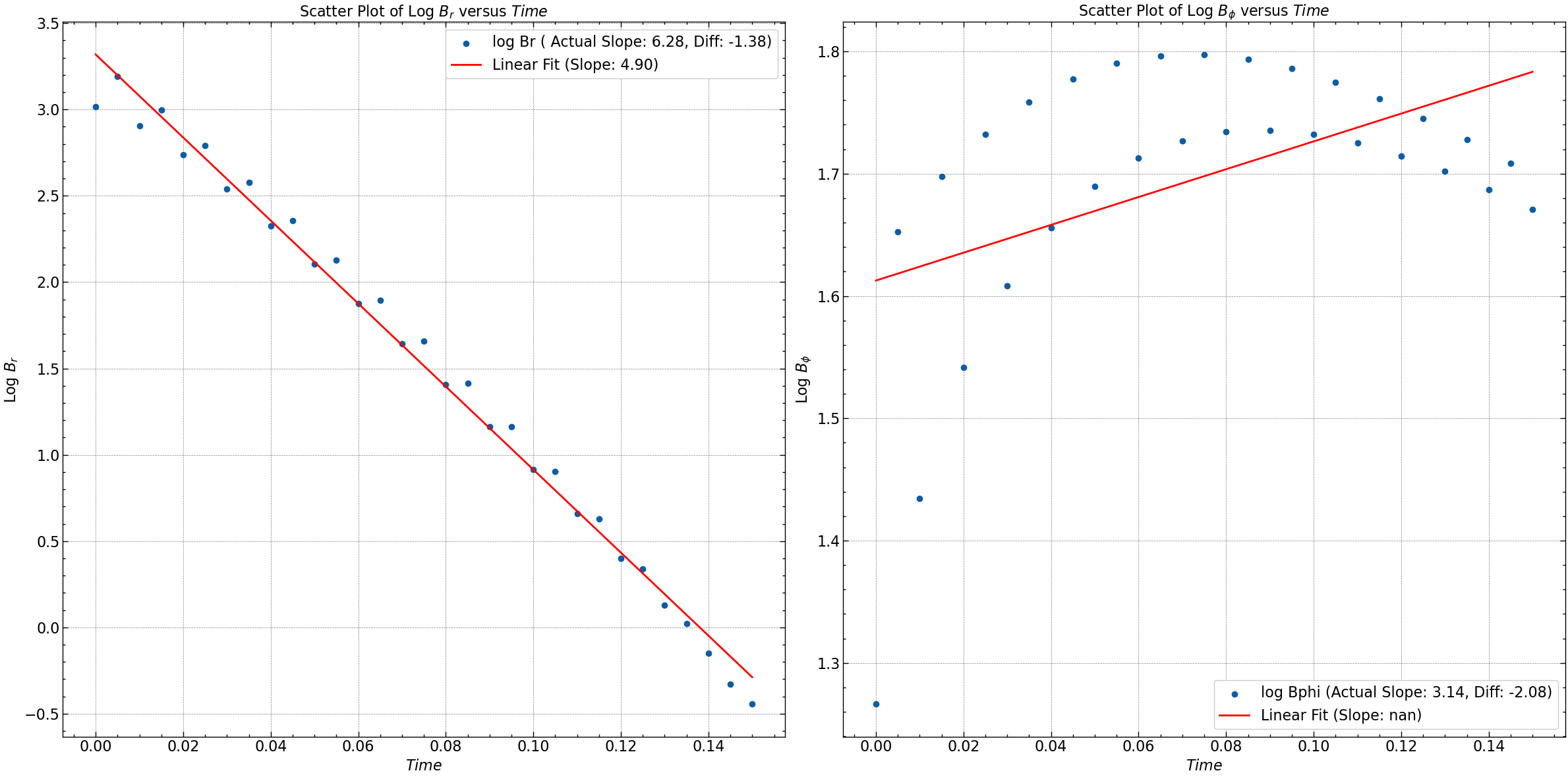
Br: Actual Slope = 6.283185307179586, Computed Slope = 4.903733737286547, Difference = -1.379451569893039
Bphi: Actual Slope = 3.141592653589793, Computed Slope = 1.0665548853197655, Difference = -2.0750377682700276

plt.figure(figsize=(24, 12))

# Scatter plot for log Br
plt.subplot(1, 2, 1)
plt.scatter(time, log_Br, label=f'log Br ( Actual Slope: {actual_slope_Br:.2f}, Diff: {difference_Br:.2f})')
plt.xlabel(r'$Time$')
plt.ylabel(r'Log $B_r$')
plt.title(r'Scatter Plot of Log $B_r$ versus $Time$')
plt.grid(True)

# Linear fit for log Br
fit_Br = np.polyfit(time, log_Br, 1)
plt.plot(time, np.polyval(fit_Br, time), color='red', label=f'Linear Fit (Slope: {np.sqrt(-fit_Br[0]):.2f})')
plt.legend()

# Scatter plot for log Bphi
plt.subplot(1, 2, 2)
plt.scatter(time, log_Bphi, label=f'log Bphi (Actual Slope: {actual_slope_Bphi:.2f}, Diff: {difference_Bphi:.2f})')
plt.xlabel(r'$Time$')
plt.ylabel(r'Log $B_{\phi}$')
plt.title(r'Scatter Plot of Log $B_{\phi}$ versus $Time$')
plt.grid(True)

# Linear fit for log Bphi
fit_Bphi = np.polyfit(time, log_Bphi, 1)
plt.plot(time, np.polyval(fit_Bphi, time), color='red', label=f'Linear Fit (Slope: {np.sqrt(-fit_Bphi[0]):.2f})')
plt.legend()

plt.tight_layout()
plt.savefig("seed_3/log_Br_Bphi_vs_time_neu.png")
plt.show()

../../_images/7ad80455d1ea28f99267463af8d95ba03eff6f9f277b330e8bdd40807a48c5c7.png